of Frequency Assignment Problems
SNEZANA PEJIC
A thesis submitted to the Department of Mathematics of
the London School of Eeonomics and Politicai Science
for the degree of Doctor of Philosophy
Déclaration
I certify that the thesis I have presented for examination for the MPhil/PhD degree of the London School of Economies and Politicai Science is solely my own work other than where I have clearly indicated that it is the work of others (in which case the extent of any work carried out jointly by me and any other person is clearly identified in it).
The copyright of this thesis rests with the author. Quotation from it is permitted, provided that full acknowledgement is made. This thesis may not be reproduced without the prior written consent of the author.
Abstract
Frequency Assignment Problems (FAPs) arise when transmitters need to be al-locateci frequencies with the aim of minimizing interference, whilst maint aining an efficient use of the radio spectrum. In this thesis FAPs are seen as generalised graph colouring problems, where transmitters are represented by vertices, and their interactions by weighted edges.
Solving FAPs often relies on known structural properties to facilitate algorithms. When no structural information is available explicitly, obtaining it from numerical data is difficult. This lack of structural information is a key underlying motivation for the research work in this thesis.
If there are TV transmitters to be assigned, we assume as given an N x N "influence matrix" W with entries Wij representing influence between transmitters i and j. From this matrix we derive the Laplacian matrix L = D—W, where D is a diagonal matrix whose entries da are the sum of ali influences working in transmitter i. The focus of this thesis is the study of mathematical properties of the matrix L. We généralisé certain properties of the Laplacian eigenvalues and eigenvectors that hold for simple graphs. We also observe and discuss changes in the shape of the Laplacian eigenvalue spectrum due to modifications of a FAP. We include a number of computational experiments and generated simulated examples of FAPs for which we explicitly calculate eigenvalues and eigenvectors in order to test the developed theoretical results.
We find that the Laplacians prove useful in identifying certain types of problems, providing structured approach to reducing the originai FAP to smaller size sub-problems, hence assisting existing heuristic algorithms for solving frequency as-signments. In that sense we conclude that analysis of the Laplacians is a useful tool for better understanding of FAPs.
Acknowledgements
It is my pleasure to acknowledge a number of people who contributed towards the successful completion of this dissertation.
First, I would like to express my sincerest gratitude to my supervisor, Jan van den Heuvel. I am grateful to Jan for introducing me to the field of spectral graph theory and for ail the unreserved support and guidance he has offered me throughout the development of this thesis.
I am extremely grateful to the whole Mathematics Department of the London School of Economies, and in particular to Norman Biggs, Adam Ostaszewski, and Bernhard von Stengel, for their enormous academic and personal support, and to Jackie Everid, David Scott and Simon Jolly for encouragement and friendship. I also want to thank Jim Finnie and Henrik Blank from the Radiocommunications Agency, with whom I cooperated in the development of this study, for their insight-ful questions, comments and suggestions, which significantly influenced, guided and motivated this work.
Throughout my éducation I received much encouragement from my family. I thank my parents for nurturing my interest and love of mathematics, and my sister Bojana for being a wonderful friend and support, even when across the océan!
Finally, I would like to thank my lovely boys, Aleksa, Sergije and Veljko, for sup-porting my efforts, and for giving me their ail important love that made this work possible and very worthwhile.
This work was funded by the U.K. Radio Communications Agency. I also give gratitude to the LSE Mathematics Department for providing an additional grant, supporting the completion of the research.
Contents
1 Introduction 6
1.1 Frequency Assignments 6 1.2 Outline of the Thesis 9
2 Preliminaries 11
2.1 Graph Theory Background 11 2.1.1 Graphs in general; simple and weighted graphs 11
2.1.2 Matrices associated with graphs 13
2.2 Linear Algebra Background 15 2.2.1 Eigenvalues and eigenvectors of matrices 15
2.2.2 Linear equations 19 2.2.3 Partitions of sets and matrices 20
2.3 Graph Theory and FAPs 22
3 Spectral Analysis of FAPs 27
3.1 Continuity of Laplacian Eigenvalues 29 3.2 Laplacian Eigenvalues of Weighted Graphs 31
3.2.1 Bounds for eigenvalues in terms of edge weights 34
3.3 Laplacian Eigenvectors of Weighted Graphs 38 3.3.1 Recognition of specific induced subgraphs 39
3.3.2 Equitable partitions 47 3.3.3 Locai properties 49 3.4 The Chromatic Number of a Weighted Graph 62
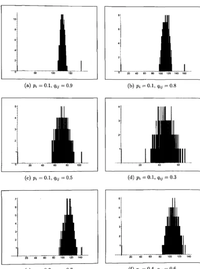
3.5 Distribution of the Eigenvalues of FAPs 68 3.5.1 FAP with one multiple-channel transmitter 68
3.5.2 The Laplacian eigenvalues of infinite grids 69 3.5.3 The Laplacian eigenvalues of finite parts of grids 71 3.5.4 Square and triangular grids with différent constraints . . . . 74
3.5.5 The Laplacian eigenvalues and specific structures 76
4 Simulated Examples of FAPs 90
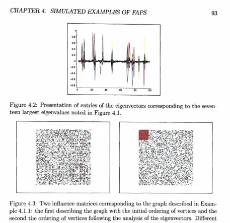
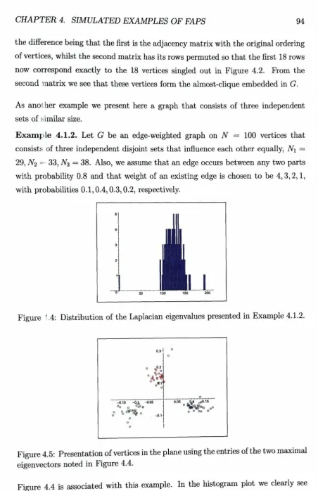
4.1 Overview of the Chapter and Introduction to the Simulations . . . 90 4.1.1 Presentation of FAPs using random graph structures . . . . 90
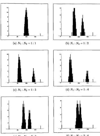
4.1.2 Introduction to the simulations 92
4.1.3 Contents of the chapter 95 4.2 Graphs with 'Regulär fc-part' Underlying Structure 96
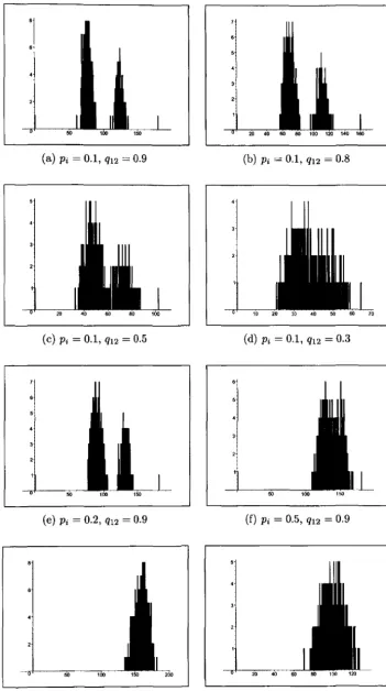
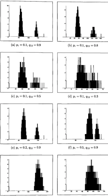
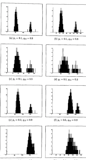
4.2.1 Two-part simulation examples with pi < qi2 97
4.2.2 Two-part simulation examples with pi > qi2 105
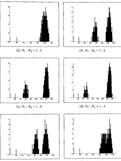
4.2.3 Three-part examples with pi < % 111 4.2.4 Four-part examples with Pi < q^ 117
4.2.5 Edge weighted graphs 119 4.3 Graphs with 'Irregulär fc-part' Underlying Structure 127
4.3.1 Graphs with two parts 127 4.3.2 Graphs with three parts 132 4.4 Towards an Interpretation of the Algebraic Properties 137
4.5 Examples with Geographie Position of Transmitters 140
Conclusion 147
Chapter 1
Introduction
1.1 Frequency Assignments
"There are very few things in the world of technology that are as finan-cially important and frustratingly arcane as the allocation and use of radio spectrum."
— The Times, lOth Aprii 2007
The challenges in the field of radio spectrum application and use lie in optimising this essential but scarce resource between numerous modem industries that dé-pend on it, whilst maintaining the technical quality and usability of each assigned frequency. The use of radio frequencies today is at the heart of the broadcast and satellite television industries, the mobile phone industry, the radio industry, numerous smaller businesses ranging from paging services to alarm monitoring companies, as well as many government services in fields such as health services, police, military, etc.
The reception quality of a signal is directly affected if the frequencies are assigned incorrectly. Spectrum allocation is constrained by the need to restrict interference between simultaneous transmissions to an acceptable level. For instance, if two services are close geographically, interference will occur if they are transmitting on frequencies which are close in the radio spectrum.
Rapid development of wireless networks in the 20th century was almost immedi-ately accompanied by allocation and planning problems requiring special considér-ation by the governments controlling the radio spectrum and frequency ownership.
In the UK, as in the US, the government partially solved the demand side of this problem by deciding to begin auctioning off spectrum once it became available for public use. In the UK, the Office of Communications (Ofcom), an independent regulator and compétition authority for the UK communications industry, is tasked to secure optimal use of the radio spectrum. A key means of achieving this aim is by releasing the available spectrum to the market, generally by means of auctions, or via the so called spectrum awards programme. The corresponding body in the US is the Federai Communications Commission.
Frequency sale has become an important source of government revenues, explaining government's active interest in the optimisation of frequency allocation. Contem-poraneously, there is an unceasing interest in optimising the use of the spectrum from the users/operators point of view.
Auctioning, nevertheless, on its own does not solve the problems related to fre-quency assignment. To make possible further improvements in spectrum availabil-ity, optimisation approaches have been used and remain fundamental.
The optimisation problems were initially confined solely to radio operators, but were eventually presented to the wider community of researchers including math-ematicians and computer scientists as well as radio engineers, who have ail found this field attractive and fruitful for research within their own disciplines. As each application created a new model, each with its own objectives and instances, the problems requiring mathematical analysis were quickly in abundance.
The main body of research into optimal spectrum allocation started in early 1960's, and has become known as the Frequency Assignment Problem (FAP). Today, the FAP is an important area of interest both in theoretical analysis and practical applications related to the development of wireless communications networks. In this thesis, frequency assignment problems are seen as problems occurring when a given set of transmitters or base stations are allocated frequencies or Channels, with the aim of minimizing interference and optimising the use of the frequency spectrum.
signal-to-noise ratio at a receiver depends on the choice of frequency, on the strength of the signal, the direction it is transmitted to, the shape of the environment, and even weather conditions. This is the reason why it is hard to obtain an accurate prédiction of the signal-to-noise ratio at receivers. The smallest tolerable ratio of wanted to unwanted signal strength is known as the protection ratio. More détails on how signal-to-noise ratio is modelled in différent research studies can be found in [1],
In our work, a convenient représentation of interference is by means of a constraint matrix W = [î%]. The quality of the service is deemed to be acceptable provided the Channels assigned to each pair of transmitters i and j are Wij Channels apart. We define this formally later in the thesis.
The main modelling variations in the application of the FAP are as follows. Fixed Channel Assignment (FCA) is a model where the set of connections remains sta-ble over time. Dynamic Channel Assignment (DCA) models allow for changes in demand for frequencies at an antenna. Hybrid Channel Assignment (HCA) Prob-lems combine the previous two: frequencies are assigned beforehand, with reserved allocation for new frequencies. In this thesis we concentrate on Fixed Channel Assignment problems.
There is a signifìcant body of work completed in attempting to tackle all the FAP related issues, with major effort put in modelling, analysis and simplification, often in solving instances of a FAP. Two comprehensive surveys on models and solution techniques and Frequency Assignments Problems in general are provided in [1] and [41]. In order to tackle the problem of spectrum congestion, one can also concentrate efforts on carefully allocating and rearranging the frequencies on which receivers and transmitters broadcast. The brauch of mathematics that is closest to this application is graph theory and in particular the area of graph colouring. The graph colouring problem is the exact field of our interest.
neu-ral networks [11, 12, 16, 18, 33, 36] have been of interest to researchers, as well as several ad hoc heuristics [14, 31, 35].
The radio community has a strong interest in the use of approximation algorithms for solving frequency assignment problems. As most of the heuristics apply to some form of neighbourhood or hyperneighbourhood search, identifying useful underlying structures within the network of transmitters under considération prior to applying the heuristic methods is valuable.
However, security and commercial reasons impose limits on information that can be revealed to the wider research community, including the information on spatial placements of transmitters. The question underlying this thesis is how much can be done in terms of analysis when no structural information is directly revealed.
1.2 Outline of the Thesis
Various methods for solving frequency assignment problems rely on the knowledge of certain structural properties to facilitate the algorithms. For instance, we may be given information about the geographical position of a set of transmitters, infor-mation about the power of the transmitters, and possibly some inforinfor-mation about the terrain properties. If no such structural information is given explicitly, it may be difficult to obtain this information from the numerical data.
We present our work as follows: In the first part of Chapter 2 we introduce the relevant notation and review ali the elementary results from graph theory that are referred to in our work. Next, we introduce the necessary results and properties from Linear Algebra. We then formally define our version of Frequency Assignment Problems in terms of graph theory, and introduce the algebraic graph theory terms: Laplacian matrices, eigenvalues and eigenvectors of the FAP.
The theoretical results related to the application of spectral analysis of the fre-quency assignment problems are presented in Chapter 3. In the introduciory sec-tion we recali the continuity of Laplacian eigenvalues which results from pertur-bation matrix theory, and explain why it provides strong support to our chosen approach to FAP analysis. Then we discuss various properties of graph Laplacian eigenvalues, focusing on extending the known results for simple graphs to the case of edge-weighted graphs.
Chapter 2
Preliminaries
In this chapter we present the mathematical terminology and notation used in our research. Initially we introduce graphs and concepts related to graphs, followed by the required concepts and basic results from matrix theory and linear algebra. Finally, we formally interpret the relation between Frequency Assignment Problems and graph theory as applied throughout our research.
2.1 Graph Theory Background
2.1.1 Graphs in general; simple and weighted graphs
By a graph G we mean a pair (V(G),E(G)), with V(G) a nonempty finite set called the vertices, and E(G) a finite collection of unordered pairs of vertices, called the edges. An edge e — uv connects or joins the vertices u and v. The vertices u and v are called the ends of e. An edge e is said to be incident to v if v is an end of e. Vertices u and v are adjacent if there exists an edge that connects them. The number of edges of which v is an end is called the degree of v and is denoted by d(v). An edge connecting a vertex to itself is called a loop. Distinct edges that connect the same pair of different vertices are called multiple edges. A graph with no loops and parallel edges is called a simple graph. In this thesis loops and parallel edges are not permitted. A regular graph is a graph where each vertex has the same degree. A regular graph with vertices of degree k is called a fc-regular graph or regular graph of degree k. Two graphs G and H are said to be isomorphic, if there
is a one-to-one correspondence, called an isomorphism, between the vertices of the graph such that two vertices are adjacent in G if and only if their corresponding vertices are adjacent in H.
A subgraph of a graph G is a graph whose vertex and edge sets are subsets of those of G. We say a graph G contains another graph H if some subgraph of G is H, or is isomorphic to H. A subgraph H is a spanning subgraph of a graph G if it has the same vertex set as G. We say H spans G. A subgraph H of a graph G is said to be induced if, for any pair of vertices u and v of H, uv is an edge of H if and only if uv is an edge of G. If the vertex set of H is the subset S of V(G), then H can be written as G[S\ and is said to be induced by S.
A walk is an alternating sequence of vertices and edges, beginning and ending with a vertex, in which each vertex is incident to the two edges that precede and follow it in the sequence, and the vertices that precede and follow an edge are the end vertices of that edge. A walk is closed if its first and last vertices are the same, and open if they are different. A walk in which all edges are different is called a trail If, furthermore, the vertices in the walk are different then the sequence is called a path. Two vertices u and v are called connected if G contains a path from u to v. Otherwise, they are disconnected. A graph is called connected if every pair of distinct vertices in the graph is connected. A connected component is a maximal connected subgraph of G. Each vertex belongs to exactly one connected component, as does each edge. The edge connectivity of a simple graph G is the minimal number of edges whose removal would result in losing connectivity of the graph G. Vertex connectivity is defined analogously (vertices together with the adjacent edges are removed). In a graph, an independent set is a set of vertices no two of which are adjacent. A clique is a set of vertices such that for every two vertices in the set, there exists an edge connecting the two.
An oriented graph is analogous to an undirected graph except that it contains only directed edges. A mixed graph may contain both directed and undirected edges; it generalizes both directed and undirected graphs. An oriented graph is called simple if it has no loops and at most one directed edge between any pair of vertices. When stated without any qualificaiion, in this thesis, we assume graphs and dia-graphs to be simple.
As a generalisation of these concepts vertex-weighted and/or edge-weighted graphs and diagraphs can be found in the literature. These are graphs with weights as-signed to their vertices and/or edges, respectively.
2.1.2 Matrices associateci with graphs
We describe several matrices that have been defined for simple graphs and dia-graphs. These have ali been of interest to algebraic graph theory. Considerable research has been devoted to trying to determine properties of graphs using alge-braic properties of these matrices.
The matrix that has been considered most often is the adjacency matrix. The adjacency matrix of a graph G ori n vertices is the n x n matrix A = [a^] whose (z, j)-entry alj is equal to the number of edges with i and j as ends.
The incidence matrix Q of a graph G is the 01-matrix with rows and columns indexed by vertices and edges of G, respectively, such that the ve-entry of Q is equal to one if and only if the vertex v is an end of edge e. It is important to note that this matrix differs from the incidence matrix for oriented graphs.
The incidence matrix Q{Gff) of an oriented graph G is the 0, ±l-matrix with rows and columns indexed by the vertices and edges of G, respectively, such that the •ue-entry of Q(Ga) is equal to 1 if the vertex v is the tail of the edge e, equal to — 1 if the vertex v is in the head of the edge e, and 0 otherwise.
In addition to these matrices we introduce the Laplacian of a graph. The algebraic approach used in this study for the analysis of FAPs relies solely on the analysis of the Laplacians.
If G is a graph on n vertices, then D{G) is the diagonal n x n matrix with rows and columns indexed by V(G), and each w-entry equal to the degree of vertex v. The Laplacian of a graph G is the matrix that represents a product of the incidence matrix and its transpose based on an arbitrary orientation of the graph G; so
L(G) = Q(G°)Qr(G°), (2.1)
where a is an arbitrary orientation of a graph G and Q{Ga) is the incidence matrix of Ga.
On the other hand one could also see the Laplacian as the différence between the diagonal matrix D(G) and the adjacency matrix A(G); so
L(G) = D(G) - A(G).
The following proposition proves that the two définitions are équivalent and that the Laplacian in the first définition is well-defined (i.e., L is independent of the orientation given to G). The proposition can be found in [9] and we include its proof for completeness.
Proposition 2.1.1. If o is an orientation of G and Q is the incidence matrix of Ga, then QQT = D(G) — A(G), where D(G) is the diagonal matrix of vertex degrees and A(G) is the adjacency matrix.
Proof. The inner product of any two rows i and j of Q corresponds to the ij-entry of QQT. If i j then these rows have a non-zero entry in the same column if and only if there is an edge e joining vertices Vi and Vj. In this case the two non-zero entries are +1 and —1 (the head and the tail of the edge e), so (QQT)ij = — 1. Similarly, (QQT)u is equal to the inner product of the row i with itself and since the number of entries ±1 in the row i is simply the degree of v¿, the resuit follows.
•
There are other "generalised Laplacians" associated with a graph. Throughout the thesis we will be referring to a version of such a generalised Laplacian for edge-weighted graphs. The formai définition is given in Section 2.3.
and v are adjacent vertices of G, and Luv = 0 when u and v are distinct and not adjacent. There are no constraints on the diagonal entries of L; in particular there is no requirement that L 1 = 0. The ordinary Laplacian is a generalised Laplacian, as is -A(G).
Chung's définition [13] refers to a "normalised" form of the ordinary Laplacian. It is denoted by C and defined as:
y/d(u)d(v ) 0,
if u — v and d(v) ^ 0, if u and v are adjacent, otherwise.
The ordinary and the normalized Laplacian are connected by the following expres-sion: C = D~1/2LD~1/2. Chung also defines a generalised normalized Laplacian for edge-weighted graphs.
2.2 Linear Algebra Background
2.2.1 Eigenvalues and eigenvectors of matrices
In this subsection we discuss a number of results from linear algebra used through-out the thesis. We begin with définitions of eigenvalues and eigenvectors for matri-ces in general. For completeness we first define Hermitian adjoint, Hermitian and normal matrices.
Let A = [dij] be a matrix over the field of complex numbers. The transpose of A, denoted by AT is the matrix over the same field as A whose entries are ci^ j that is, rows are exchanged for columns and vice versa.
The Hermitian adjoint A* of A is defined by .4* = (Ä)T, where Ä is the entry-wise conjugate.
Definition 2.2.1. A complex square matrix A is a Hermitian (or self-adjoint) matrix if it is equal to its own conjugate transpose, i.e., A = (Ä)T.
matrix, i.e., if it is symmetric with respect to the main diagonal. A real and symmetric matrix is simply a special case of a Hermitian matrix.
Definition 2.2.2. A complex square matrix A is a normal matrix if A*A = AA* where A* is the conjugate transpose of A.
It should be added that if A is a real matrix, A* = AT and so it is normal if ATA = AAT. Every Hermitian matrix, and hence every real symmetric matrix is normal.
Definition 2.2.3. Let A be an n x n matrix over the field of complex numbers. We consider the equation
Ax = Ax, x ^ 0,
where x is an n-vector and A is a scalar. If a scalar A and a non-zero vector x happen to satisfy this equation, then A is called an eigenvalue of A and x is called an eigenvector of A associated with A.
The set of ali eigenvalues is called the spectrum of A. The space of eigenvectors of A associated with the eigenvalue A together with the nuli vector is called the eigenspace belonging to A. The dimension of this space is called the geometrie mul~ tiplicity of A. On the other hand, the algebraic multiplicity of A is the multiplicity of A as a root of the polynomial det(4 — XI). For Hermitian matrices the two mul-tiplicities of A are equal. As both the graph adjacency and Laplacian matrix are Hermitian we, in this work, need not distinguish between geometrie and algebraic multiplicity and speak solely about the multiplicity of an eigenvalue.
Since in this thesis we only analyse matrices associated with graphs there is an additional refinement. Note that rows and columns of the adjacency and Laplacian matrix are indexed by the vertices of the considered graph G. This implies that we can view these matrices as linear mappings on EV{G), the space of real functions on V(G). If f € MV(G) and A is the adjacency matrix of G, then the image Af of
/ under A is given by
(Af)(u)= £ Auvf(v),
vev(G)
and since A is just a 01-matrix we have:
If we suppose that / is an eigenvector of A with eigenvalue A, then Af = A/, and so
A/(«0 = £ / ( « ) .
Any function that satisfies this condition is an eigenvector of A.
Below we list several known facts for symmetric and positive semidefinite matrices. These are standard results from linear algebra (see, e.g., [28]).
Proposition 2.2.4. Let A be a real nxn symmetric matrix. Then
• two eigenvectors of A with different eigenvalues are orthogonal;
• all eigenvalues of A are real numbers;
• Rn has an orthonormal basis consisting of eigenvectors of A.
A real symmetric matrix A is positive semidefinite if xTA x > 0 for all vectors x. If x is an eigenvector of A belonging to an eigenvalue A then xTAx = \xTx, which implies that a real symmetric matrix is positive semidefinite if and only if its eigenvalues are nonnegative. For this class of matrices we also know:
Proposition 2.2.5. A real symmetric matrix A is positive semidefinite if and only if there is a matrix B such that A = BBT.
Moving our attention on to a particular matrix, the Laplacian matrix L, the previ-ous two properties help determine that L is positive semidefinite (see equation (2.1) on page 14) implying that its eigenvalues are real and non-negative.
Next, we introduce the concepts of interlacing and tight interlacing of sequences. Consider two sequences of real numbers: Ax > ... > An, and /x i > ... > ßm with
m <n. The second sequence is said to interlace the first one whenever
A i> ßi> An_m+i for i — 1 ,. . . , m.
The interlacing is called tight if there exists an integer k G [0, m] such that
Ai = fa for 0 < i < k and An-m+i = for k -f 1 < i < m.
The interlacing inequalities become Ai > /zi > A2 > /¿2 > • • • > ßn-i > An, when
Now, assume that the sequence
A i 0 4 ) > A2( A ) > . . . > An( , 4 ) ,
represents the eigenvalues of a Symmetrie matrix A in decreasing order, and let the coordinates of the matrix and corresponding vectors be indexed by a set V, where \V\ = n. A useful characterisation of the eigenvalues is given by the Rayleigh's and Courant-Fisher's formulae (see [39]):
\n{A) = min{<,4x,z} | x e Rv, ||®|| = 1},
Ai (4) = max{ (Ax,x) \ x G Rv, ||z|| = 1},
An-fe+i(-4) = min{max{ (Ax,x) \ x G X, \\x\\ = 1} |
X a fc-dimensional subspace of Rv }, for k = 1 ,. . . , n.
Also,
An_fc_j_i(^4) = min{ (Ax,x) \ = 1, x _L Xi for i = n — k + 2,...
where xn, ... are pairwise orthogonal eigenvectors corresponding to An, An_i,..., An_fc+2, respectively.
For the purposes of the our work we single out one of the many important applica-tions of this characterisation to eigenvalue interlacing between eigenvalues of two matrices.
Proposition 2.2.6. Let A and B be Hermitian n x n matrices. Assume that B is positive semidefinite and that the eigenvalues of A and A + B are arranged in decreasing order. Then
\k{A)<\k(A + B),
for ail k = 1,..., n.
Before we proceed further we include one more property that we refer to later, which does not involve interlacing, but describes another useful relation between eigenvalues in the case of commuting matrices.
permutation i\,..., in of the indices 1,..., n, such that the eigenvalues of A + B are ai + /3h, a2 + Aa,...,an -I- (3in.
In the following chapters we use these two properties. These, together with many other matrix analysis results, can be found in any standard textbook on matrix theory (e.g, [28]).
2.2.2 Linear équations
Consider a linear transformation L : V W, where V and W are vector spaces. One of the problems in linear algebra is that for a given vector b G W one wants to find ali vectors a € V such that L(a) = b. Usually, this is written in the form
L(x) = 6,
and is referred to as a linear équation (with functional part L, free member b and unknown x).
Equivalently, consider a matrix équation with a coefficient AÌ a free member B and unknown X , where
AX = B,
and A and B are matrices over the same scalar field K that have the form:
A
-«11 a12 OLin
«2i Oi22 a2n
«ml «m2 ' " ' «mn
' A " Xi
,
B = P2 X2,
B = P2 :Jm _ xn
It is obvious that the solutions of this matrix équation are the solutions of the system of linear équations with m linear équations and n unknowns over the scalar field K. In fact, the matrix équation can be seen as a linear équation
LA(X) = B
the set of ail its solutions is an affine subspace of K n
R(A, B) = a + A 0)
where R(A, 0) represents the vector space of ail solutions of its corresponding ho-mogenous system AX = 0. Furthermore, similarly to the previous case, we have dim R(A, B) =n- rank (A). Also:
Proposition 2.2.8. A system of m linear équations with n unknowns over the scalar field K has at least one solution if and only if the matrix A and the augmented matrix [A\B] are of the same rank.
This property implies that a system of linear équations over the scalar field K has exactly one solution if and only if rank ([A\B]) = rank (A) = n, where n is the number of unknowns. In particular we have:
Proposition 2.2.9. A homogenous system of linear équations, i.e., a matrix équa-tion AX — 0 has a non-trivial soluéqua-tion X ^ 0 if and only if the rank of the matrix A is smaller than the number of unknowns n.
2.2.3 Partitions of sets and matrices
A partition 7r of a set 5 is a set whose elements are themselves disjoint nonempty subsets of S, and whose union is S. The elements of the partition are called parts or cells and by 7T = ( 5 i , . . . , Sm) we mean a partition with m cells, the fc-th of which is Sk• The partition with ail cells containing exactly one element is called
discrete, and the partition with one celi trivial.
For a partition ir of S we construct vectors of size whose entries correspond to elements of S, and hence to the entries of the cells. If entries of such a vector are equal to 1 on ail elements of the celi Sk and equal to 0 otherwise, then we cali such a vector the characteristic vector of the celi Sk of partition ir.
Similarly, a partition ir of S can be presented by its characteristic matrix P = [pij], which is defined to be the |5| x m matrix with characteristic vectors of the cells as its columns:
Note that PTP is a diagonal matrix where (PTP)kk = |£fc|- Since the cells are nonempty, the matrix PTP is invertible.
A block matrix, or a partitioned matrix is a partition of a matrix into rectangular smaller matrices called blocks. The matrix is written in terms of smaller matrices written side-by-side. A block matrix must conform to a consistent way of Splitting up the rows, and the columns: we group the rows into some adjacent 'bunches', and the columns likewise. The partition is into the rectangles described by one bunch of adjacent rows crossing one bunch of adjacent columns. The matrix is split up by some horizontal and vertical lines that go ali the way across.
Assuming that rows and columns of a square n x n matrix A are both partitioned according to the partitioning 7r, partitioning of A can be presented as
An ' ' ' m A = ! : ,
A , ... A
where Aij is a submatrix of A, whose rows are indexed by Si and columns by Sj. Definition 2.2.10. The quotient matrix of a matrix A partitioned according to n is the matrix Q whose entries are the average row sums of the blocks of A. More precisely Q — [%•] is such that
1 T 1
Qij — 1T Aj 1 = AP)ij.
Definition 2.2.11. The partition is called equitable if each block A^ of A has constant row (and column) sum, that is, AP = PQ.
Below we list interesting facts and results on interlacing of eigenvalues of matrices. We start with a classical and fundamental case of interlacing by Courant (see [15]).
Proposition 2.2.12. Let A be a real Symmetrie n x n matrix, and let S be a complex n x m matrix (n > m) such that S* S = Im. Set B equal to S* AS and let {î/i? • • • j Vm} denote an orthogonal set of eigenvectors of B. Then
• If fa = K or Hi = An_m+i for some i Ç [1 ,m], then there exists an
eigen-vector y of B with eigenvalue fa, such that S y is an eigeneigen-vector of A with eigenvalue
• If the interlacing is tight, then SB — AS.
A proof of the theorem and the corollaries that follow can be found in [22, 26]. We single out two inieresting conséquences.
Corollary 2.2.13. Let A be a real nxn symmetric matrix. The maximum of the quadratic form tr(XTAX) on XTX = Ik is the sum of the k largest eigenvalues of the matrix and the nxk matrix X giving the maximum contains the corresponding eigenvectors in its columns.
Proposition 2.2.14. Let A be a Hermitian matrix partitioned as follows
A\\ • • • Aim A = ; i ,
AMI ' ' ' AMM
such that An is square for i = 1,... Let bij be the average row sum of Ai j, for — 1,... ,m. Define the m x m matrix B to be a matrix whose (i,j)-entry is equal to btj for ail values of i and j. The following holds:
• The eigenvalues of B interlace the eigenvalues of A.
• If the interlacing is tight, then A is equitable.
• If for i,j = 1,... , m, Aij has constant row and column sums, then any eigenvalue of B is also an eigenvalue of A with at least as large a multiplicity.
2.3 Graph Theory and FAPs
In this thesis we discuss the possibility of using algebraic techniques to investigate the structure of frequency assignment problems, using numerical data such as a constraint matrix only.
To explain our approach further, we first describe some of the underlying assump-tions.
Frequency assignment problems can be described in différent ways, using différent collections of information. We will always assume that we are given a collection of N transmitters, numbered 1 , N .
What is further available may vary depending on the specific problem. For instance, we may have access to information about the géographie position of the set of transmitters, information about the power of the transmitters, or information about the terrain properties.
For our purposes we assume that ail we have available is the constraint matrix: Definition 2.3.1. A constraint matrix W = [wij] is an N x N matrix such that if fi denotes the frequency assigned to transmitter i, for i = 1,..., N, then in order to limit interference it is required that \ fi — fj\ > Wij, for ail
We use the term "transmitter" in a general sense, as a unit assigned with one Channel. In a system where certain "actual transmitters" need to be assigned more than one Channel, we will consider each channel as a separate "transmitter". This makes sense because a transmitter with multiple Channels is indistinguishable from a system where there is a number of transmitters ali in more or less the same position.
We will also use the term influence matrix for the constraint matrix. After all, the constraint that needs to be imposed between two transmitters to manage the interference is directly related to the influence they have on one another.
Definition 2.3.2. A feasible assignment of a FAP with N transmitters, given the constraint matrix W, is a labelling f : { 1 ,. . . , N} —> { £ € M | £ > 0 } such that Ifi - /il > Wij, for ail i j , i ± j.
Accepting the hypotheses in the définitions above, the constraint matrix is the unique object needed to "solve the FAP".
The main purpose of the methodology discussed here is to obtain further informa-tion about the FAP, which may be helpful to existing algorithms used.
For several reasons, including historical developments of solution methods for FAPs, we will usually discuss FAPs in the context of weighted graphs.
Définition 2.3.3. A weighted graph (G, w) is a triple (V(G), E (G), w), where V(G) and E(G) form the vertex set and edge set, respectively, of a simple graph G, and w is a weight-function defined on E(G). We will assume that ail weights w(e), e G E(G), are non-negative real numbers.
In order to simplify notation we use G to denote a weighted graph.
Also, we treat the situation that there is no edge between two vertices u and v and the situation where there is an edge uv with w(uv) = 0 as équivalent.
In an edge-weighted graph, an independent set would be a set of vertices no two of which are adjacent, or equivalently a vertex set where every two are connected with an edge of weight 0. A clique would then be a set of vertices such that for every two vertices in the set, there exists an edge of non-zero weight connecting the two.
If a FAP with the constraint matrix W = [?%-] is given, then we can easily form a weighted graph G by setting = { 1 , . . . , AT}, joining two vertices i,j whenever Wij > 0, and setting the weight of an edge e = ij equal to w(e) = Wij. Similarly, given a weighted graph, we can formulate a FAP on the vertex set in the reverse manner.
From now on we will mix both FAPs and weighted graphs, and hence we talk about the span of a weighted graph G, notation sp(G), as the span of the related FAP. We also use a mixture of FAP-terms and graph theoretical terms. Therefore a vertex and a transmitter should be considered as being the same object.
The chromatic number x(G) °f a graph G is the smallest number of labels needed
As indicateci previously, we always assume that a weighted graph G has an associ-ated matrix W. We define the (weighted) degree of a vertex v as d(v) = w(uv). Définition 2.3.4. Given a weighted graph G with associated matrix W, denote by D the diagonal matrix with the degrees of the vertices on the diagonal. Then we define the Laplacian L of G as the matrix L = D — W; hence
(here, and in the définition of degree above, wefollow our convention that w(uv) = 0
If we want to emphasise the weighted graph G determining the Laplacian we denote the Laplacian as L(G).
The matrix L can be seen as a généralisation of the Laplacian matrix from algebraic graph theory, in a similar way that W is a généralisation of the adjacency matrix of a graph.
Note that the information contained in the Laplacian is the same as that in the con-straint matrix. In that sense, there seems to be no good reason to study algebraic properties of the Laplacian instead of the constraint matrix. However the Lapla-cian is more useful in obtaining structural information in relation to the underlying graph (or the FAP). It also has additional algebraic properties (for instance, it is positive semidefinite) which give us a headstart in the algebraic analysis.
There are, however, some (but quite spécifie in description) graphs for which there is a direct connection between the spectrums of the constraint matrix and the spectrum of the Laplacian. Those are generalised edge-weighted regular graphs with ali edge weights equal and ali vertices of constant degree A. For those graphs we have: \ ( L ) = -Ai(W) + A.
Définition 2.3.5. Given a weighted graph or a FAP with the Laplacian L, a Laplacian eigenvalue and a Laplacian eigenvector is an eigenvalue and eigenvector of L. So X e M is a Laplacian eigenvalue with corresponding Laplacian eigenvector x G RN if x ^ 0 and Lx = Xx.
Since L is a symmetric matrix (Luv = Lvu) we know it has N rea! eigenvalues u^v
—w(uv), ifu=£v, d(v), ifu = v
Ai,..., Ajv, and a collection of corresponding eigenvectors xu... ,xN that form a basis of RN. Because of the fairly nice structure of the Laplacian, determining
the eigenvalues and eigenvectors is computationally fairly uncomplicated, even for larger values of N. Experiments with N « 10,000 have been performed on a standard PC, where running times were in the order of minutes.
The guiding question in the remainder of this thesis is:
Chapter 3
Spectral Analysis of FAPs
Modem spectral theory is widely used in ail areas of science where a certain prop-erty can be described by connections and relations within a structure.
In theoretical chemistry the adjacency matrix eigenvalues are thoroughly investi-gated and used in revealing the properties and the structure of atoms, molecules and molecule groups [17].
Spectral theory in the past found a rôle in the theory of electrical networks, where the matrix of interest was the so called matrix of admittance or conductivity. From that time we have Kirchhoff's theorem (1847), a well-known theorem that shows that the number of spanning trees in a graph is equal to the déterminant of the matrix obtained from the Laplacian by removing one row and column corresponding to the same vertex [32].
The différence Laplacian, a variant of the Kirchhoif matrix, is the matrix of a quadratic form expressing the energy of a discrète system. It also naturally de-scribes the vibration of a membrane, or thermodynamical properties of crystalline lattices. The discrète analogue shares many important properties with its contin-uons version, undoubtedly the most important and best understood operator in mathematical physics.
Spectral techniques are applied in computer science in information retrieval and data mining (see, e.g., [4]). There they are used to cluster documents into areas of interest, and to determine the relative importance of documents based on some underlying structure. Web information retrieval is one of the main examples. The
web's hyperlink structure has been exploited by several of today's leading Web search engines, particularly Google [34].
Researchers also applied spectral techniques in observing the autonomous systems of the internet. An autonomous system is a collection of Internet Protocol (IP) networks and routers under the control of one entity (or sometimes more) that présents a common routing policy to the Internet. Their adjacency spectrum was investigated in [19], and the normalized Laplacians in [42].
Researchers also applied spectral techniques in observing the autonomous systems of the Internet. Informally, an autonomous system (AS) is a single network or a group of networks under a single administrative control. An example of an au-tonomous system might be the set of ail computer networks owned by a university, or a company. Their adjacency spectrum was investigated in [19], and the normal-ized Laplacians in [42].
The research in graph theory in recent years has focused on the Laplacian spectrum in an attempt to design approximation algorithms for NP-hard problems, such as graph partitioning, graph colouring and finding the largest clique in a graph. Fiedler [20] was among the first to study the properties of the second smallest Lapla-cian eigenvalue (called Fiedler eigenvalue), its corresponding eigenvector, and their relationship to the Connectivity of a graph. He observed [21] that the différences in the components of this eigenvector are an approximate measure of the distance between the vertices. Alon and Millman [3] looked at the relationship between the Fiedler eigenvalue and the isoperimetric number which is related to the problem of computing good edge separators. Barnes [7] suggests an algorithm for partitioning the nodes of a graph. Ali these pieces of research closely relate to the research topic of clustering mentioned earlier.
Numerous other problems have been solved using Laplacians. Barnard, Pothen and Simon [6] use the Laplacian matrix for envelope réduction of sparse matrices, while Juvan and Mohar [30] use this eigenvector to compute bandwidth and p-sum reducing orderings. Mohar and Poljak [40] provide a comprehensive survey of the applications of the Laplacian spectra to combinatorial problems.
Overall, it has been shown successfully that the Laplaeian spectrum has many attractive theoretical properties which give it a fundaraental rôle in spectral theory. In this chapter we discuss the relevance of the theoretically derived results about the Laplaeian eigenvalues (and in particular their eigenvectors) in algebraic graph theory and FAPs. The work presented includes, is motivated by, and at the same time is an extension of our published joint work [25].
3.1 Continuity of Laplaeian Eigenvalues
The following properties from perturbation theory of matrices are important in our research. They support our idea that one can classify FAPs according to their similarities, i.e., slightly changed initial information in the influence matrix should not change the approach to solving a given problem. This becomes extremely important when we recognize that a new problem can be compared to an "almost similar problem" for which we have previously developed a method for solving. Since we are currently interested in the spectrum of Laplaeian matrices, our in-tention is to draw conclusions about the behaviour of the spectrum when certain small changes are introduced.
We will be working with vector and matrix norms described below. Let x = [xi,..., xn]T dénoté a vector of size n, and let A = [ai7-] dénoté an n x n matrix.
Définition 3.1.1. The vector fa-norm (the Euclidian norm) on Cn is defined by
Définition 3.1.2. The matrix l2-norm (the Probenius norm) on Cn is defined by
We define a new term, the eigenvalue vector.
Our aim is to prove that slight changes in the Laplacian matrix cause small changes to its eigenvalue vector. In other words:
Theorem 3.1.4. Let T be the operator that maps the set of symmetric matrices into the set of vectors, such that the image of a matrix is its eigenvalue vector.
Then T is a continuous operator.
The following theorem and its corollary are needed:
Theorem 3.1.5. (Hoffman and Wielandt) Let A and E be n x n matrices, such that A and A +E are both normal, let {Aj,..., An} be the eigenvalues of A in some given order, and let {À'x,..., AJJ be the eigenvalues of A + E in some order. Then
there exists a permutation a of the integers 1,2,..., n such that
1/2
< P l h L i=1
For Hermitian matrices, and therefore for the real symmetric ones that we are concerned with, this theorem is used to prove a stronger resuit stated below. The proof of the theorem and the corollary can be found in [28].
Corollary 3.1.6. Let A and E be n x n matrices, such that A is Hermitian and A + E is normal, let {Ai,..., An} be the eigenvalues of A arranged in increasing order (Ai < A2 < ... < An), and let {AJ,..., AJJ be the eigenvalues of A + E ordered so that Re < Re \'2 < ... < Re\'n. Then we have
È w
-. i= 1Proof. According to Theorem 3.1.5, there is some permutation a of the given order (increasing real parts) for the eigenvalues of A + E for which
. ¿=1
If the eigenvalues of A + E in the list A^(1),..., A'a(n) are already in increasing order
of their real parts, there is nothing to prove. Otherwise, there are two successive
< Il
eigenvalues in the list that are not ordered in this way, so
K(k) > ^(fc+i) f°r some k , 1 < k < n.
But since
\K{k) — Afc|2 + Ià^j.j) — Afe+i|2 =
= _ -f |A^(fe) - Afc+i|2 + 2(Afc - Xk+i)(Re A^fc+1) - Re A^(fc)),
and since A* — Afc+i < 0 by assumption, we see that
l^affc) — Xk\2 + — Afc+i|2 > |A^fc+1) — Afc|2 + |A'a(fc) — Afc+i|2.
Thus, the two eigenvalues and can be interchanged without increasing the sum of squared différences. By a finite sequence of such interchanges, the list of eigenvalues . . . , can be transformed into the list A'l5 A'2,..., A'n in which
the real parts are increasing and the asserted bound holds. •
For Hermitian matrices A and B and their eigenvalues arranged in increasing or decreasing order we have
¿ l A ^ - A ^ f i=1
1/2
<U-B
||
2| and this is exactly the relation that proves Theorem 3.1.4.3.2 Laplacian Eigenvalues of Weighted Graphs
In this section we talk about bounds for the Laplacian eigenvalues in terms of the number of vertices and the number of components of weighted graphs.
The results that follow are inspired by known theorems for simple graphs (see, e.g., [5, 23, 38]).
Proof. It is easy to see that L 1 = 0, (each row sum of L is 0), so we conclude that 0 is a Laplacian eigenvalue of the graph.
Let x be any vector orthogonal to 1. Then we easily obtain Lx = (cN)x. Since there are exactly N — l linearly independent vectors orthogonal to 1, cN is a
Laplacian eigenvalue with multiplicity N - 1. •
We recali the définition of weighted graph, Definition 2.3.3. There we note that we regard the situation of no edge between two vertices u and v and that there is an edge uv of weight 0 as identical. We are now ready to define the complément of an edge-weighted graph.
Définition 3.2.3. The complément (G,w) (or just G) of a weighted graph G is the weighted graph with the same vertex and edge set, and with weights w(e) = C—w(e) for an edge e G E(G), where C = max wie).
e€E(G)
Theorem 3.2.4. If X is a Laplacian eigenvalue of a weighted graph G on N vertices and maximal edge-weight C, then 0 < À < CN.
A vector orthogonal to 1 is an eigenvector of the Laplacian L(G) corresponding to the eigenvalue A if and only if it is an eigenvector of the Laplacian L(G) of the complément G corresponding to the eigenvalue CN — A.
Proof. Let G be a weighted graph with M edges. Choose an orientation of the edges of G. The vertex-edge incidence matrix Q of G is the N x M matrix Q such that
y/w(e), if edge e points toward vertex v,
Qve = —y/w(e), if edge e points away from vertex v, 0, otherwise.
Note that this means that L(G) = QQT
-For an eigenvalue A ^ 0 of the Laplacian L there exists a vector x, with ||x|| = 1, such that Lx = Xx. Thus A = (\x,x) = (Lx,x) - (QQTxix) = {QTx,QTx) =
||QTa:||2. Therefore A is real and non-negative.
to 1, then according to Lemma 3.2.2 we have:
L(G)x = L(K^)x-L(G)x = {CN - X)x. (3.1)
Since the Laplacian eigenvalues of G are also non-negative, we get A < CN.
Expression (3.1) also proves the last part of the theorem. • Theorem 3.2.5. Let G be a weighted graph with N vertices and maximal
edge-weight C. The multiplicity of the eigenvalue 0 equals the number of components of the graph and the multiplicity of the eigenvalue CN is equal to one less than the number of components of the complementary graph G.
Proof. We define the incidence matrix Q as in the previous proof, and without loss of generality we assume that the first m rows of the incidence matrix Q correspond to the vertices of a component of G of order m. The sum of these rows is 0T and
any m — 1 rows are independent. This means that the rank of the matrix formed from these m rows is m — 1 and hence its nullity is 1. Therefore, each component of the graph contributes 1 to the the nullity of Q. Since the nullity of Q is the same as the nullity of QQT (and hence, of L), we conclude that the nullity of L(G) is equal to the number of components of the graph. In other words, the multiplicity of the Laplacian eigenvalue 0 equals the number of components of the graph. This proves the first part of the theorem.
Furthermore, from Theorem 3.2.4, we know that for each eigenvalue CN of L(G) with associated eigenvector that is orthogonal to 1, there is one eigenvalue 0 of L(G) associated with the same eigenvector. Since in the Laplacian spectrum of any graph there is one eigenvalue 0 that is associated with all-1 vector 1, we deduce that the value CN is an eigenvalue of L(G) with multiplicity k if and only if 0 is an eigenvalue of L(G) of multiplicity +1. According to the first part of the theorem, the latter is true if and only if G has k + 1 components. This completes the proof.
•
Definition 3.2.6. The complete A;(c)-partite graph ^jv^,...,^ ™ the weighted
Theorem 3.2.7. Let G be a weighted graph on N veriices and maximal edge weight C. Then the multiplicity of CN as an eigenvalue of the Laplacian ma-trix L is equal to k — 1 if and only if G contains a complete k-partite graph ^Ni,...,^ as a spanning subgraph ofG.
Proof. According to Theorem 3.2.5 the multiplicity of CN is equal to k - 1, one less the number of components of the complementary graph G. On the other hand G has k components if and only if G has a complete fc(c)-partite graph Nk
as a spanning subgraph.
3.2.1 Bounds for eigenvalues in terms of edge weights
In this subsection we prove certain results concerning bounds for the smallest non-zero and the largest Laplacian eigenvalue of a weighted graph. Throughout the section let G be a weighted graph on N vertices and suppose its Laplacian L has eigenvalues ordered as follows:
0 = ^n(L) < \n~I(L) < • • • < Ai(L).
We recali the Rayleigh's and Courant-Fisher's characterisation of the eigenvalues on page 18, which implies that for the second smallest eigenvalue of a weighted graph G with the Laplacian matrix L we can write:
XN-I(L) = min{ (Lx,x) | ||a;|| = 1 , re _L 1 } , (3.2)
since 1 is the eigenvector corresponding to the minimal eigenvalue XN(L) = 0. Theorem 3.2.8. Let G be a weighted graph on N vertices. Then we have
1
Ajv-1 < w(uv) + - (d(u) + d(v)),
Proof. Choose two vertices u,v, u ^ v, and define a vector with real entries x — [a?i,..., XN]t as follows:
Xi =
1, if i — u, —1, if i = V,
0, otherwise.
As vector x is orthogonal to 1, from expression (3.2), we have (Lx,x) (Lx)Tx d(u) + d(v) + 2 w(uv)
AN-I S —, v- = —^— = ,
x1 x 2
which proves the theorem. •
From this theorem the following corollary may be obtained.
Corollary 3.2.9. If a weighted graph has at least one pair of non-adjacent ver-tices u,v, then XN-i < \ (d{u) + d{v)) < \ (dmax + dmax) = dmax, where dmax denotes the maximum degree.
Note that the value of XN-I can be greater than dmax in the case of a weighted graph in which any two vertices are adjacent. For example, ÀN- I ( K $ ) = cN > c(N - 1) = dmax(Ktf).
Definition 3.2.10. The 2-degree c^M of a vertex v of a weighted graph G is the sum of the degrees of its neighbours times the weight of the edge with which v is joined to that neighbour. So d2(v) = w(uv)d(u).
Theorem 3.2.11. Let Xi be the largest Laplacian eigenvalue of a connected weighted qraph G with no isolated vertices. Then Xi < max \d(v) + ^f } }.
v€V(G)1 d(v) J
To prove Theorem 3.2.11, we use Gersgorin's Theorem and its corollaries. These are classical results regarding the location of eigenvalues of général matrices, and can be found in, e.g., [28].
Theorem 3.2.12 (Gersgorin's Theorem). Let A = [%] be an N x N matrix,
and let N
dénoté the deleted absolute row sums of A. Then ali the (complex) eigenvalues of A are located in the union of N dises
N
|J{ z € C | |z - Otfl < RfiiA)} = G(A). i=1
Furthermore, if a union of k of these N dises forms a connected région in the complex plane that is disjoint from ail other N — k dises, then there are precisely k eigenvalues of A in this région.
Corollary 3.2.13. Let A = [ay] be an N x N matrix and let
N
C'jiA) = J2 hil. i =
denote the deleted absolute column sums of A. Then ali the (complex) eigenvalues of A are located in the union of N dises
z € C \ \z — AJJ\ < Cj(A) } = G(AT).
Furthermore, if a union of k of these N dises forms a connected région that is disjoint from ail other N — k dises, then there are precisely k eigenvalues of A in this région.
Theorem 3.2.12 and Corollary 3.2.13 together show that ali the eigenvalues of A lie in the intersection of the two régions, that is, in G(A) D G(AT).
Corollary 3.2.14. If A — [a+j] is an N x N matrix, then
N N max{ |À| | A an eigenvalue of A} < minj max ^ |oy|, m a x ^ |a»j| j .
j=l 3 i=1
We are now ready to give a proof of Theorem 3.2.11.
the matrix defined by
d(u), if u = v,
(D 1LD)UV = < d(v)/d(u), if there is an edge joining u and u, if u = v
0 otherwise.
V
Since D is invertible, D 1LD has the same eigenvalues as L. Therefore, application of Corollary 3.2.14 to the rows of D~lLD gives us
Fiedler [20] looked to characterise simple graphs by means of the spectra of the Laplacian matrix. He is well-known for naming Ajv-i the algebraic Connectivity
of a simple graph, because of the relation with two common concepts from graph theory: edge and vertex Connectivity of the graph. That work produced a couple of inequalities that easily généralisé to edge-weighted graphs which we use later in the thesis. The following are the original Fielder results rewritten for edge-weighted graphs.
Theorem 3.2.15. Let G be a weighted graph on N vertices. Then
where Ô(G) denotes the minimal, and A (G) denotes the maximal generalised vertex
degree.
Proof. For a weighted graph G, with the Laplacian matrix L (which is positive semidefinite) we know
and hence the resuit follows.
NS(G)
and
Atf_i(L) = min{ (Lx,x) \ ||z|| = 1, x J_ 1},
which implies
Let
L = L-Xn^(I-N~1J)ì
where J is the N x N all-one matrix. We show that L is positive semidefinite. Let y be any vector in RN. Then y can be written in the form y = al + ßxt a and ß scalars, ||x|| = 1, and x IX. Since ¿1 = 0, it follows that
yTly = ß2xTLx = ß2(xTLx
-which is obviously non-negative according to earlier observations. Thus the mini-mum diagonal entry of L is nonnegative
min. (Lü - XN-ÎH - N"1)) > 0, 1 <I<N
which in graph theory terms is exactly équivalent to
Ö(G)-XN_1{1-N~1)>0.
Furthermore, according to Theorem 3.2.4 the following relation between the maxi-mal Laplacian eigenvalue of G and the second minimaxi-mal Laplacian eigenvalue of the complément holds
X1(G) = CN-XN-1(G),
where C denotes the largest edge weight in G. We note from Definition 3.2.3 that ö(G) = C(N — 1) — A(G), and hence, as in the previously proved inequality for Ajv-i (G) we have
XL(G) > C N - I ^ = C N - N { C { N ~ V ~ A { G ) ) =
1V iV-1 N — 1 N — 1
3-3 Laplacian Eigenvectors of Weighted Graphs
a full collection of eigenvectors, we can reconstruct the matrix. Therefore we can expect to obtain more detailed information about a FAP by considering both the eigenvalues and certain eigenvectors simultaneously. Eigenvectors themselves are sometimes observed through their entries and we note that each entry corresponds to exactly one vertex of the graph. Since the Laplacian matrix is Symmetrie, all the entries can be taken to be real numbers.
3.3.1 Récognition of specific induced subgraphs
Earlier we presented a couple of known results for eigenvalues of weighted graphs. For instance, the number of components is equal to the multiplicity of the Laplacian eigenvalue 0, and we saw that the multiplicity of CN is related to the existence of the induced complete fc-partite graph. In our first interaction with eigenvectors we investigate if the entries of the eigenvectors that correspond to particular Laplacian eigenvalues can reveal more about the graph itself. The results follow.
Theorem 3.3.1. Let G be a weighted graph on N vertices. The multiplicity k of the Laplacian eigenvalue 0 i$ equal to the number of components of G.
If each component has Ni vertices, i = 1,..., k, then the values of Ni and the ver-tices in each component can be recognised as follows: The N x k matrix M whose columns are the k independent eigenvectors corresponding to the eigenvalue 0 con-tains k différent rows m^, i = 1,..., k, where row m® occurs Ni times. Moreover, the indices of the identical rows correspond to vertices belonging to the same com-ponent of G.
Proof. Theorem 3.2.5 already explains that the multiplicity of the eigenvalue 0 represents the number of components of the corresponding weighted graph.
Let us, therefore, focus on the second part of the theorem that states the relation between coordinates of the eigenvectors and the components of the graph. Consider the matrix M, described in the statement of the theorem, where we propose that identical rows of M correspond to vertices of the same component.
to the second component, etc. We define the vector X to be a vector that is constant on the entries of the k components of the graph. The Laplacian matrix L and the vector X can be represented as follows:
" Lu 0 0
0 L22 i
, X = X2
• 0
, X =
0 0 Lkk
where Lu is an Ni x Ni submatrix that represents the Laplacian matrix of the i-th component of G, whilst Xi is a subvector of size Ni with entries corresponding to the z-th component of G.
It is easy to prove that LX ~ QX (the row sum of each of the Lu matrices is 0), and since there are exactly k linearly independent choices for X, we can conclude that any such choice gives a basis of the Laplacian eigenspace that corresponds to the eigenvalue 0. This also means that a matrix that has these k eigenvectors as its columns is such that it contains at most k différent rows of which the first Ni are identical (equal to say), the second iV2 are identical, (equal to ra(2)), etc.
for any choice of k independent eigenvectors. In fact, this matrix has exactly k distinct rows, for the rank of the matrix is k. This proves the existence of a bijection between the rows of the matrix M and the vertices of G so that indices of the identical rows are the indices of the vertices that belong to the same component
of the graph G. • Theorem 3.3.2. Let G be a weighted graph on N vertices and of maximal edge
weight C. The graph G contains a complete k^-partite graph K^ Nk as a span-ning subgraph if and only if the multiplicity ofCN as an eigenvalue ofthe Laplacian matrix L is k — 1.
Furthermore, the N x (k — 1) matrix M whose columns are the k — 1 independent eigenvectors that correspond to the eigenvalue CN contains k différent rows
i = 1,..., k where each row m ^ occurs Ni times. Moreover, indices of identical rows correspond to the vertices belonging to the same part Vi of the k^-partition of G.
a spanning subgraph. The main point for discussion here is the remaining part of the theorem, describing the relationship between entries of the eigenvectors and the partition of vectors.
In order to assess which vertices of G belong to which part, we consider the k — 1 independent eigenvectors that correspond to CN. More precisely, we look at the matrix M described in the statement of the theorem. Our claim is that identical rows of M correspond to vertices in the same part.
In order to do this, consider the complementary weighted graph G. Following Theorem 3.2.4, we see that G has a Laplacian eigenvalue 0 of dimension k, and ail eigenvectors of L(G) for the eigenvalue CN are also eigenvectors of L(G) for the eigenvalue 0. Additionally, the all-1 vector 1 is an eigenvector of L(G) corre-spondis to the eigenvalue 0. Using this information in Theorem 3.3.1 immediately reveals that G has a structure consisting of k components, where the vertices of each component can be found by looking at identical rows in the matrix of eigen-vectors (the extra vector 1 makes no différence here). Going back to the original
graph G, this means a structure for G as described in the theorem. •
Corollary 3.3.3. Let L be the Laplacian of a FAP with N channels, where the maximal interference between any pair is C. Then the two following statements are équivalent:
1. The system contains a partition Si, £2,..., of the channels into k parts of size Ni, i = 1,..., k, with the property that the interference between any pair of vertices from différent parts is C;
2. There is a Laplacian eigenvalue CN of multiplicity k — 1 such that the k — 1 corresponding eigenvectors have the following form:
• they are orthogonal to 1;
• the N x (k — 1) matrix M whose columns are the k — 1 eigenvectors contains k différent rows i = 1,... ,k, where each row mfi occurs Ni times.
These first observations are useful to check if a given FAP can be divided into independent FAPs of smaller size, and whether a given set of transmitters can be split into subsets where the vertices of différent subsets influence each another maximally.
The results instantly give hope that we should be able to use Laplacian eigenvalues and eigenvectors in the analysis of the underlying structure of a graph. Theo-rem 3.4.5 in the next section will show that the knowledge about the structure of a FAP along the lines of the corollary above, can be very useful when trying to find the span of the FAP. However, other connections are generally not so easily spotted. That is the reason why our research is initially directed to considering several graphs with specific structures and their Laplacians, and only then do we move to more realistic cases, where we explore ideas on how to use the Laplacians. The following theorem explores whether a given set of transmitters can be separated into subsets where the vertices from différent subsets influence one another with an average weight w. By this we mean that for the given two subsets of vertices the following holds: for any vertex the average of edge weights between the vertex and ali the vertices in the other subset is w.
Theorem 3.3.4. Let G be a weighted graph on N vertices. Suppose there is a non-zero Laplacian eigenvalue wN of multiplicity k — \, and iftheNx(k-l) matrix M, formed from k — 1 independent eigenvectors corresponding to the eigenvalue wN,
contains k différent rows m^, i = where each row m^ occurs Ni times, and where one ofthem have ail entries equal to 0. Then G contains k vertex disjoint subgraphs that cover V(G) that influence one another with an average weight w. Moreover, indices of rows that are identical correspond to vertices belonging to the same subgraphs of G described above.
Proof. Without loss of generality we present the k — 1 eigenvalue-eigenvector équations in form of a matrix équation L(G) M = wN M, i.e.,
' L<") L<12> L(lk)
-¿(21) £(22)
l
_ £( f e l ) L(kk)
M™
M<
2>
M
(fc)= wN
MM
M(
2)
AfW
Here, by M ^ we dénoté an Ni x (A; — 1) submatrix of M with ail rows equal to and by L^ an Ni x Nj submatrix of L containing information about the influence between Ni vertices corresponding to the rows equal to ra^ and Nj vertices that correspond to rows equal to m W e present the entries of m ^ as
(0 fmW
7ïiy 1 = m 1 5 m^lj, and we write Ri(A) when referring to the i-th row of some matrix A.
Our aim is to show that the average of the elements in the rows/columns of the matrices i ^ j is equal to value —tu. First, we prove it for the first row of L by considering the équation
R^VjM^wNR^M). (3.4)
We dénoté the sum of entries of the r-th row of L ^ by By taking the transpose of both sides of équation (3.4), using the property that the columns of M are orthogonal to 1, and simplifying the équation obtained we get:
(2) (1)
m;' — m
(1) (2)
mk-1 - K-1
(1) (2) ml ml
m ( i )
fc-i m (2) fc-i
= wN
(i) m) — m
(i)
raJUi - m (k) k-1
m (i)
m ( i ) fc-i
(1) (k)
m\ - m\
( i )
K - i - m k-1
where X is a transpose of Ri(L), the first row of L, with the first N\ entries omitted. This équation is équivalent to
(i) (2)
m\' — m\
(1) (2)
(i) (*) m\ ' — m\'
(i)
mk-1 ~ mk-1 J
" z<12) " ' wNmS11 "
_ x[lk) _ wNm^li
Since the rank of
m\ — m\
(1) (2) K-i - TOfc-i
(i) <fc) m ' — m '
(i) (*) ti/ATra^
tüJVm^
is the same as the rank (k — 1) of
(1) (2)
ml ml
(1)
™>k-l ~ m fc-1 (2)
(1) (fc)
mj — mj
(i) - m (k) fe-i
and since it is equal to the number of unknowns k—1, we conclude that the équation has exactly one solution and that one soluti