FOR COMPATIBLE WIND SPEED
ESTIMATION
Benjamin PIPER
Acoustics Research Centre
School of Computing, Science and Engineering
University of Salford, Salford, UK
List of Tables and Figures...I Acknowledgements...IX Abstract...X
1. Introduction...1
1.1 Statement of The Problem...2
1.2 Introduction...3
1.3 Previous Studies in SODAR Operation, Comparison, and Accuracy Testing ...3
1.3.1 Outline of the Development of SODAR Instruments...3
1.3.2 Motivation for use in Wind Energy...6
1.3.3 SODAR Comparison Studies...7
1.3.3.1 Comparison Studies Specifically Aimed at Wind Energy Requirements ...11
1.3.4 SODAR Comparisons with Transponder Based Simulated Echoes ...16
1.3.5 Methods to Measure Contributing Aspects of a SODAR's Acoustic Beam Pattern...19
1.3.6 Summary...21
1.4 Overview of the Acoustic Operation of SODARs...21
1.5 Statement of the Aims of This Thesis...25
1.5.1 The UpWind Project...27
1.6 Outline of Methods to Explore SODAR Measurement Uncertainty...28
1.7 Summary...28
2. Theoretical Comparison of Known Differences Between SODARs...30
2.1 Introduction...31
2.2 Far-field Model of Sound Radiation from 2D Speaker Arrays...32
2.3 Measurement Volume Differences...37
2.4 Effect of Sound Frequency on SODAR Measurements...46
2.4.1 Effect of Frequency on the FWHM of the SODAR Beam...46
Background Noise of SODAR Measurements...48
2.5 Effect of Beam Tilt Angle...52
2.5.1 Wind Speed Resolution in a Single Measurement...52
2.6 Potential Fixed Echo Influence Based on Side Lobe Pattern and Baffle Shape. 54 2.6.1 Side Lobe Position and Magnitude...54
2.6.2 Diffraction of the SODAR Beam by Baffle Edges...59
2.7 Influence of Peak Detection and Averaging Processes...61
2.8 Doppler Shift Equations...63
2.9 Measurement Rejection Algorithms...67
2.10 Discussion...67
2.11 Summary...68
3. A Transponder System As A Method For Comparing SODARs...70
3.1 Introduction...71
3.1.1 Principle of Transponder Measurements...71
3.2 Physical Design of Transponder System...71
3.2.1 Transponder Sound Sources...72
3.2.2 Transponder Input Microphone...76
3.2.3 Transponder Laptop...78
3.2.4 Transponder Set-up...78
3.3 Transponder Processing...79
3.3.1 The Input Stage...79
3.3.2 Analysis of the SODAR Signal...79
3.3.3 Constructing the Return Signal...81
3.3.3.1 Synthesis...82
3.3.3.2 Modulation...82
3.3.3.3 Wind Speed Profiles...83
3.3.4 Amplitude Envelope...84
3.3.5 The Output Stage...86
3.6 Laboratory Testing of Transponder System...90
3.6.1 Methodology...90
3.6.2 Results from Testing with METEK DSDPA.90-24...92
3.6.2.1 Test One - Vertical Speed Estimation ...92
3.6.2.2. Test Two– Constant Wind Speed Profiles...94
3.6.2.3. Test Three – Changing Wind Speed Profiles...100
3.6.2.4. Test Four – Constant Wind Speed Profiles in Presence of White Noise ...104
3.6.3 Measurements with the AQ500 SODAR...105
3.6.4 Discussion...106
3.7 Field Testing of Transponder System...107
3.7.1 Details of the Specific Problems Faced by the Transponder in a Field Situation...107
3.7.1.1 The Real Atmospheric Echo ...107
3.7.1.2 Background Noise ...108
3.7.1.3 Impulsive Wind Noise on the Microphone ...108
3.7.1.4 Physical Structure ...108
3.7.2 Adapting the Transponder for Use in the Field...108
3.7.2.1 Portable Anechoic Chambers ...109
3.7.2.2 Dome Frames and Tents ...109
3.7.2.3 Arched Framework ...110
3.7.2.4 Gazebo Frames ...111
3.7.3 Field Measurement Results With a METEK DSDPA.90-24 at Carrington (UK)...111
3.7.3.1 Test Two – Constant Wind Speed Profiles...112
3.7.3.2 Test Three – Changing Wind Speed Profiles...113
3.7.3.3 Summary...113
Calibration Tool...117
3.8.1 Making the Return Echo More Realistically...118
3.8.2 Removing the Real Atmospheric Echo...118
3.9 Summary...118
4. Methods to Measure the Beam Shape and Tilt Angle of SODARs...120
4.1 Introduction ...121
4.2 Anechoic Measurements of SODAR Horns...121
4.2.1 Measurement Methodology...122
4.2.2 Measurement Results and Analysis...122
4.2.3 Summary...124
4.3 Anechoic Measurements of SODAR Arrays...124
4.3.1 Measurement Methodology...124
4.3.2 Measurement Results and Analysis...126
4.3.3 Summary...128
4.4 Near Field Acoustic Holography (NAH) to Measure SODAR Directivity ...128
4.4.1 NAH Principle...129
4.4.2 Investigations into the Prediction of a SODAR's Far-Field Directivity Using NAH...130
4.4.3 Investigations into Measuring and Predicting Baffle Edge Interference Using NAH...132
4.4.4 Summary...134
4.5 In-Field Directivity Measurements Using a Tilting Platform...135
4.5.1 Methodology ...136
4.5.2 Results and Analysis...139
4.5.2.1 Results Recorded without the SODAR's Baffles...139
4.5.2.2 Results Recorded with the SODAR's Baffles...142
4.5.3 Conclusions...144
4.6 Beam Tilt from SODAR data (Bradley Method) ...145
4.6.3 Conclusion ...149
4.7 Discussion ...149
4.8 Summary ...153
5. Method Integration and Further Work...155
5.1 Introduction...156
5.2 Hypothetical Example of the Application of the Research Findings...156
5.2.1 The SODAR, Turbine and the Measurement Site...157
5.2.2 Results...158
5.2.3 Summary of Hypothetical Example...164
5.3 Implications for Wind Energy Measurements with SODARs...166
5.3.1 How Does the Proposed SODAR Comparison Method Fit into the UpWind Project?...167
5.4 Specific Further Work to Realise Comparison Methods for SODARs...168
5.5 Summary...169
6. Conclusions ...171
...178
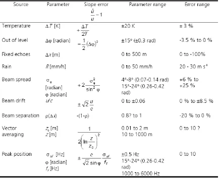
Table 1.3.1 – Table of the error contribution from various aspects of a SODAR's measurement
process. Bradley (2005)...12
Table 1.3.2 – Regression Coefficients from the PIE Measurements. Bradley (2005)...13
Figure 1.3.1 – Variation in regression slope with height for the measurements of a METEK (Δ), a AV4000(+) and a Scintec(O) SODAR made in the PIE from Bradley (2005)...14
Figure 1.3.2 – Flow Diagram of the Acoustic Pulse Transponder designed for USEPA quality assurance and detailed in Baxter (1994 a & b)...18
Figure 1.4.1 – Amplitude Vs Angle Function, ka.sin(θ), of a First Order Bessel Function...22
Figure 1.4.2 – Wave Front Shape of a SODAR Reflection...22
Figure 2.2.1 – Directivity pattern, Hs, for a single circular source...33
Figure 2.2.2 – Directivity function, Hc for a column of 4 point sources with a separation of 8cm at 4.5 kHz with no Beam shift applied (solid) and a 15° shift applied (dashed)...34
Figure 2.2.3 – Calculation of the directivity (H) of a 4*4 square array using the directivity of its layout (Hc) and source type (Hs)...35
Figure 2.2.4 - Two examples of speaker array layouts...36
Figure 2.2.5 – Comparison of the 4.5 kHz directivity of three different array shapes using identical sources showing across the arrays' Y-Axis (solid), diagonal (dashed) and X-Axis (dotted)...36
Table 2.3.1 – Angular width and cross sectional area at 100m for 3 SODAR array shapes for sound at 4.5 kHz...38
Figure 2.3.1 – Source of coefficients for calculating ERVP...39
Figure 2.3.2 – Example of curve fitting to find X coefficient for the square shaped array...40
Figure 2.3.3 – Signal multiplied by the Gaussian window used to calculate ERVP...41
Table 2.3.2 – The ERVP and the coefficients used to calculate it for the 3 SODAR array shapes...41
Figure 2.3.4 - Calculation of volume of air passing a turbine. ...43
10ms-1 ...44
Figure 2.3.5 – Ratio of the volume measured by 3 SODAR array shapes to the volume passing a turbine example for the 10m range gate centred at 100m...44
Figure 2.3.6 – Ratio of the whole profile volume measured by 3 SODAR array shapes to the total volume passing a turbine example...45
Figure 2.4.1 – FWHM as a function of frequency for three different array shapes...47
Figure 2.4.2 – Scattering cross section as a function of frequency for a ground temperature of 10ºc at the ground (solid) and at a height of 250m (dashed)...48
Figure 2.4.3 – Absorption as a function of frequency for relative humidity values of 0% to 100% with a constant temperature of 10ºC and pressure of 101.3 kPa...49
Figure 2.4.4 - SPL Drop off as a function frequency for a reflection from 200m due to spherical spreading and atmospheric absorption for relative humidity values of 0% to 100% with a constant temperature of 10ºC and pressure of 101.3 kPa...50
Figure 2.4.5 – Signal SPL above background noise of SODAR signals reflected from 200m for relative humidity values of 0% to 100% with a constant temperature of 10ºC and pressure of 101.3 kPa...51
Figure 2.5.1 - Resolution of the horizontal wind speed estimation from one tilted beam as a function of tilt angle for a single measurement. ...53
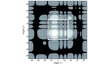
Figure 2.6.1 – Contour map in Cartesian projection of the directivity pattern of a 4*4 square array with above -6dB (white), above -20dB (light grey) above -50dB (grey) and below -50dB (black) contour areas shown and with A white square to represent a typical baffle aperture.. .56
Figure 2.6.2 – Contour map in Cartesian projection of the directivity pattern of a 12 element diamond array with above -6dB (white), above -20dB (light grey) above -50dB (grey) and below -50dB (black) contour areas shown and with a white square to represent a typical baffle aperture...56
Figure 2.6.3 – Contour map in Cartesian projection of the directivity pattern of a 3*4 staggered rectangle array with above -6dB (white), above -20dB (light grey) above -50dB (grey) and below -50dB (black) contour areas shown and with a white square to represent a typical baffle aperture...57
Figure 2.6.4 – Contour map in Cartesian projection of the directivity pattern of a 4*4 square array with a 15º tilt applied. Above -6dB (white), above -20dB (light grey) above -50dB (grey) and below -50dB (black) contour areas shown and with a white square to represent a typical baffle aperture...58
Figure 2.6.6 – Diffraction behaviour at SODAR baffle edge with sound rays represented by black arrows...60
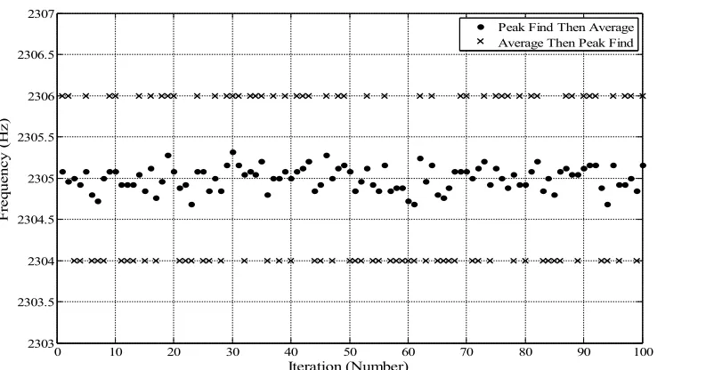
Figure 2.7.1 – Comparison between the peak frequency estimation for 100 iterations of averaging 50 signals using peak find then average (dots) and average then peak find (crosses) for signals centred at 2305 Hz...63
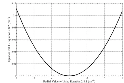
Figure 2.8.1 – Difference between the radial velocities calculated from equation 2.8.1 and 2.8.2...65
Figure 2.8.2 – Difference between the horizontal velocities calculated from Equation 2.8.1 and 2.8.2 assuming 0ms-1 vertical velocity...66
Figure 3.2.1 – Measured directivity patterns of a RCF horn loudspeaker at 2300 Hz (Left) and 4500 Hz (Right)...72
Figure 3.2.2 – Polar response of the A5-2 panel in 28mm enclosure, Azima (1999)...73
Figure 3.2.3 – Measured directivity of VISITON SC 4 ND tweeter loudspeaker...74
Figure 3.2.4 - Auto spectra of 3 VISITON SC 4 ND tweeter loudspeakers measured on axis at a distance of 1m for 2.83V input...75
Figure 3.2.5 – Geometry of sound incident on SODAR ARRAY...75
Figure 3.2.6 – Nearfield limit vs frequency for 4 commercially available SODARs with manufacturers suggested operation frequency or frequency range marked with star symbols.77
Figure 3.2.7 - Transponder set-up for measurements with a METEK DSDPA.90-24...78
Figure 3.3.1 – Extraction of the signal envelope using a Hilbert function...81
Figure 3.3.2 – Wind speed profiles used in transponder processing to generate return echo signals...84
Table 3.3.1 – Atmospheric values used in the transponder system...85
Figure 3.3.3 – Envelope used in the transponder processing for 1500 Hz (dot-dash), 3000 Hz (dot), 4500 Hz (dashed) and 6000 Hz (solid) input signals...85
Figure 3.4.1 – Example of results recorded when using an early version of the transponder system with a METEK DSDPA.90-24 SODAR. Data shown is in METEK Grafik software format with time in 30 minute divisions along the X axis and horizontal U vector wind speed in 1 ms-1 divisions along Y axis...87
(right) when using synthesis to generate transponder return signals...88
Figure 3.4.3 – Difference between transponder horizontal input speed and the all height mean of SODAR measured horizontal speed in easterly direction (left) and northerly direction (right) when using SSB modulation to generate transponder return signals...89
Table 3.6.1 – Mean difference and standard deviation of 5 tested vertical velocities over the complete data set recorded...93
Figure 3.6.1 – Mean and standard deviation of the difference between the transponder input speed and the SODAR measured speed for each range gate height and input speed...93
Figure 3.6.2 – Difference between transponder input speed and SODAR measured speed in vector components U and V for spectral and cluster averaging methods...94
Figure 3.6.3 - Difference between transponder input speed and SODAR measured speed in vector components U and V for spectral and cluster averaging methods after difference in Doppler equation is accounted for...95
Figure 3.6.4 – Differences in U component at individual heights for each transponder input speed using spectral averaging...96
Figure 3.6.5 - Average difference in U component at individual heights for each transponder input speed using cluster averaging...97
Figure 3.6.6 - Difference between transponder input speed and SODAR measured speed for horizontal vector component U for two separate averages using the cluster averaging method (First average-dashed, second average-dotted)...97
Figure 3.6.7 – Difference between the transponder input speed and the SODAR measured speed using spectral averaging for the U component of the horizontal wind speed at three different frequencies (1900 Hz – dotted/circle, 2100 Hz – dashed/cross, 2300 Hz –
dot-dash/square)...98
Figure 3.6.8 – Difference between the transponder input speed and the SODAR measured speed using cluster averaging for the U component of the horizontal wind speed at three different frequencies (1900 Hz – dotted/circle, 2100 Hz – dashed/cross, 2300 Hz –
dot-dash/square)...99
Figure 3.6.9 – Mean measured wind profiles and the difference between the transponder input speed and the SODAR measured speed for the U component of the horizontal wind speed. 100
Figure 3.6.10 – Mean measured wind profiles and the difference between the transponder input speed and the SODAR measured speed for the V component of the horizontal wind speed...101
horizontal components and wind direction...101
Figure 3.6.12 - Measured profiles and difference between transponder input speed and SODAR measured speed of the U component of the horizontal wind speed for profiles based on an Ekman spiral model...102
Figure 3.6.13 - Measured profiles and difference between transponder input speed and SODAR measured speed of the V component of the horizontal wind speed for profiles based on an Ekman spiral model...103
Figure 3.6.14 – Difference between SODAR measured speed and transponder input speed for averages with white noise added to the transponder signal with amplitudes of 1% to 80% in relation to the peak echo amplitude...104
Figure 3.6.15 – Example of spectrum recorded with AQ500 SODAR when testing with transponder system...106
Figure 3.7.1 – Examples of dome tent structures that could be used to house the transponder system in a field situation (Left to right – Large Dome Tent, Geodesic Greenhouse, Garden Yurt)...109
Figure 3.7.2 – Arch structure that could be used to hold the transponder components in
position above a SODAR...110
Figure 3.7.3 – Difference between transponder input speed and SODAR measured speed for measurements of the components of the horizontal wind speed made outside at Carrington with the METEK SODAR using spectral averaging only...112
Figure 3.7.4 – Mean measured wind profiles and the difference between the transponder input speed and the SODAR measured speed for the U component of the horizontal wind speed. 113
Figure 3.7.5 – ASC4000 Wind Explorer SODAR set-up at Wind Test Grevenbroich's turbine testing field in Germany. ...115
Figure 3.7.6 – Differences between transponder input speed and SODAR measured speed using an ASC4000 SODAR in its initial orientation. ...116
Figure 3.7.7 – Differences between transponder input speed and SODAR measured speed using an ASC4000 SODAR in its altered orientation...117
Figure 4.2.1 – Measured directivity patterns of two loudspeakers compared to a prediction from a piston function based model...122
Figure.4.3.2 – Measured directivity patterns of METEK DSDPA.90-24 SODAR array for 2200 Hz and 4500 Hz in horizontal and diagonal axis...126
Figure 4.3.3 – Anechoically measured SODAR array directivity compared with modelled directivity across horizontal axis for a frequency of 2200Hz...127
Figure 4.4.1 – NAH measured directivity patterns of METEK DSDPA.90-24 SODAR array from Taylor (2009)...131
Table 4.4.1 – Estimated FWHM of SODAR beam based on Figure 4.4.1...132
Figure 4.4.2 – Position of NAH measurement plane and projection planes in relation to SODAR baffle...133
Figure 4.4.3 - Sound radiation patterns from a SODAR baffle edge predicted from NAH measurements at different heights in relation to the baffle edge height...133
Figure 4.4.4 – Proposed NAH measurement geometry for measuring aspects of SODAR directivity including baffle diffraction effects with holography measurement planes shaded. ...135
Figure 4.5.1 – Set-up of tilting platform for measurements of the SODAR array beam shape. ...137
Figure 4.5.2 – Position of SLM in relation to SODAR array mounted on tilting platform....138
Figure 4.5.3 – Raw data from measurements of METEK DSDPA.90-24 SODAR directivity using a tilting platform and without baffles attached...140
Figure 4.5.4 – Measured directivity of METEK DSDPA.90-24 SODAR array using tilting platform method for a tilted and untilted SODAR beam compared with modelled beam patterns of the same array shape...141
Figure 4.5.5 – Measured data for tilted SODAR beam fitted with a quadratic curve to estimate the acoustic tilt angle...142
Figure 4.5.6 – Measured directivity of METEK DSDPA.90-24 SODAR array with full baffles using tilting platform method for a tilted and untilted SODAR beam...143
Figure 4.5.7 – Measured data for tilted SODAR beam with baffles fitted with a quadratic curve to estimate the acoustic tilt angle...144
Table 4.6.1 – Comparison between estimated beam zenith angles and the calculated zenith angle for results presented in Bradley(2010)...145
averages...148
Table 4.6.2 – Mean beam tilt angle and difference between SODAR reported angle for beams 1 and 2...148
Figure 5.2.1 – Array layout of example SODAR array...157
Figure 5.2.2 – Example measurement site layout...158
Figure 5.2.3 – Directivity pattern of example SODAR at 3600 Hz based on a source size of 12.2cm...159
Figure 5.2.4 – Ratio of effective volume measured by the SODAR example to the volume passing the wind turbine over a 10 minute period assuming the SODAR makes 150 samples in the same period...160
Figure 5.2.5 – 2D directivity pattern of the SODAR array tilted by 16º in Cartesian projection with the baffle edge position marked by a white square...161
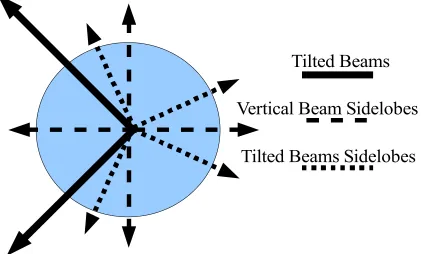
Figure 5.2.6 – Side lobe direction guide applied to site map with side lobes marked by bold dashed arrows...162
Figure 5.2.7 – Corrections to SODAR measured wind speed to give estimation of the wind speed at the turbine based on both the acoustic beam tilt angle and the effective beam tilt angle...163
I would like to thank my supervisor Sabine von Hünerbein for all her support, knowledge and guidance. Without her help and encouragement I would not have finished this thesis. I would also like to thank Stuart Bradley and Paul Behrens for their enthusiastic input and discussions from the other side of the world. I am grateful for the financial support and the feedback received at meetings of the UpWind project.
Thanks to Windtest Grevenbroich, in particular Qi Wang and Monika Krämer, for allowing and helping me to carry out transponder measurements in very snowy conditions at their wind turbine testing field in January 2010. Also I would like to thank Kenneth Underwood and Gunter Warmbier for their discussion of the outcomes of these measurements.
A big thank you to everyone in the acoustics department at Salford University. There have been many people who have lent me equipment, offered me their
knowledge and given me crucial encouragement throughout. In particular I would like to thank David Waddington, Andy Moorhouse, Paul Kendrick, Matthew Taylor, Tomos Evans, Andy Elliot and Richard Hughes. Finally I am hugely thankful for all the
This thesis includes the results of a PhD study about methods to compare Sonic Detection And Ranging (SODAR) measurements to measurements from other
instruments. The study focuses on theoretical analysis, the design of a transponder system for simulating winds and the measurement of the acoustic radiation patterns of SODARs. These methods are integrated to reduce uncertainty in SODAR
measurements.
Through theoretical analysis it is shown that the effective measurement volume of a range gate is 15% of a cone section based on the SODAR's Full Width Half Maximum (FWHM). Models of the beam pattern are used to calculate the ratio of air passing a turbine to that measured by a SODAR over 10 minutes with values of 3-5% found at 10ms-1
. The model is used to find angles where significant Sound Pressure Levels (SPLs) occur close to a SODARs baffle giving the highest chance of fixed echoes. This is converted into an orientation guide for SODAR set-up.
The design of a transponder system is detailed that aims to provide a calibration test of the processing applied by a SODAR. Testing has shown that the transponder can determine the Doppler shift equation used by a SODAR although further work is needed to make the system applicable to all SODARs.
It is shown that anechoic measurements of single elements are useful for improving array models. Measurements of the FWHM and acoustic tilt angle can be achieved in the field using a tilt mechanism and a Sound Level Meter (SLM) on a 10m mast. The same mechanism can be used to calculate an effective tilt angle using the Bradley technique.
1. Introduction
1.1 Statement of The Problem
SODARs are useful tools for measuring aspects of the atmospheric boundary layer (ABL) such as wind speed and turbulence. In the early stages of their
development they were employed to measure the height of the boundary layer by recording the strength of the return echo. By employing several beams in a
complimentary arrangement it is possible to solve a set of simultaneous equations to give the wind speed and direction at many points within the measurement height range.
There are some uncertainties in SODAR measurements that need to be overcome. Uncertainties in SODAR measurements can be divided into uncertainties caused by the measurement target and uncertainties caused by the SODAR itself. Uncertainties caused by the measurement target cannot be directly dealt with but methods to minimise their effect can be developed. Uncertainties caused by the SODAR itself can be dealt with and methods to remove these altogether are needed. These uncertainties include incorrect beam tilt, flaws in peak detection, incorrect height estimation, fixed echoes, broadband and tonal noise errors and incorrect handling of strong atmospheric shears. There is a statistical mismatch between measurements from different SODARs because most SODARs use different geometries and processing methods to achieve a wind estimation. Whilst these
methods are similar an understanding of how measurements using different SODARs correlate together is required.
The main motivation for improving the accuracy and understanding of SODAR measurements is their potential use in the wind energy market. With increasing
anemometers and wind vanes have been used to collect data for these purposes. A SODAR could be a useful alternative providing many measurements throughout the turbine height without the need to build expensive masts. In order for SODAR to be a
'bankable' measurement instrument for wind energy a means of reducing and
confirming the uncertainty in the measurements is required.
1.2 Introduction
In this Chapter previous SODAR comparison work will be explored along with a brief overview of the acoustic operation of SODARs. How SODAR measurements relate to wind energy will be explained with the required accuracy of the wind industry identified. The state of the art for SODAR measurements and comparison methods will then be stated with reference to previous work carried out to qualify the accuracy and meaning of SODAR measurements. The work in this thesis forms part of the UpWind project and follows on from the Wind Energy SODAR Evaluation (WISE) report which is reviewed in depth here. The research questions and the aims of this thesis are stated with an outline of the proposed approach.
1.3 Previous Studies in SODAR Operation, Comparison, and Accuracy
Testing
1.3.1 Outline of the Development of SODAR Instruments
the movement of turbulent reflectors. This frequency shift gives the wind speed along the direction of the SODAR measurement beam known as the radial wind speed. Bi-static types are described in Georges (1972), Beran (1973), Gaynor (1977) and Davey (1978) and they operate with an output antenna and several receiving antenna
separated by a distance. The advantage of this set-up is a gain in the strength of the reflection due to the contribution of both velocity inhomogeneities and temperature inhomogeneities. The disadvantage is that they are difficult to set-up due to the large space separation between antennas. Single axis mono static SODARs are only capable of measuring along beam wind velocity but this is useful for air quality studies since the transport of gases in the ABL follows the vertical velocity. Examples of their use can be found in Caughey (1976) and Helmis (1985). The use of a mono-static SODAR or psuedo-mono-static SODAR featuring multiple antennas tilted in a complimentary arrangement allows for a set of simultaneous equations to be solved that gives an estimation of the horizontal wind speed and direction. Examples of this SODAR type can be found in Neff (1986), Elisei (1986) and Finkelstein (1986).
The SODARs discussed so far have tended to be large and heavy instruments that operate at lower frequencies with ranges of up to 1km. From the late 1970s smaller high frequency SODARs have been developed based on early work found in Mousley (1979) on the use of arrays of speakers . These SODARs are often referred to as mini-SODARs as they tend to be smaller than previous instruments allowing them to be easily transported and set up. Examples of these are described in Asimakopoulos (1987 and 1996) and Mursch-Radlgruber (1993a and b) . This capability of mini-SODARs makes them of interest to fields where wind speed and direction at a range of heights in the lower ABL, around 150-300m, are needed such as wind energy.
described in Underwood (2010) and Scott (2010). There are several different
companies that produce SODARs with these features specifically aimed at the needs of wind energy. These SODARs represent the state of the art in commercially available SODAR instrumentation.
There are several experimental SODARs that are under development that aim to determine whether large changes in the method employed by a SODAR can give better quality results. The bi-static SODAR type that was initially used in the 1970s is
redeveloped in Behrens (2008) making use of modern computer processing power to allow for the receivers to scan the SODAR beam though the use of a Fourier-domain shifting technique. The option of integrating this into a commercially available mono-static SODAR as an add on component is detailed in Bradley (2010a). The possibility of using coded frequency pulses to obtain more detailed information than can be
achieved through single frequency pulses was discussed in Bradley (1999). Rao (2009) makes comparison between measurements made with a coded multi-frequency pulse and a single frequency pulse referenced to high resolution GPS sonde balloon
measurements showing that the use of coded pulses improves the signal to noise ratio giving 30% more wind data and with a higher consistency observed. Von Hünerbein (2010) takes the coded pulse principle further presenting a SODAR design that also allows for complete control of all sound producing elements giving control of the beam steering. The aim of this experimental SODAR is to make use of intelligent data analysis methods to give significant gains in signal to noise ratio and data quality and an advanced atmospheric model has been created in Kendrick (2010) to test this idea.
The complexity and wind estimation ability of SODARs is improving at a steady pace but a 'black box' approach is required to confirm their uncertainty levels before they will be accepted by the wind energy industry. This approach would allow a user to ensure the quality of their data without requiring the manufacturer to publish proprietary details about the operation of the SODAR in question.
aeroplane wing wake vortex measurements as demonstrated in Bradley (2007), air quality studies shown in Gera (1990) and Emeis (2006) and meteorological research with a discussion made in Kallistratova (2004). Whilst these disciplines have less stringent demands than the wind energy industry they would also benefit from a reduction in measurement uncertainty.
1.3.2 Motivation for use in Wind Energy
Recent growth in the wind energy market makes SODAR an attractive alternative measurement technique to previous tools due to their relative cost and portability advantages. From the 1990s onwards the number of wind farms and the size of the turbines used in these farms has continued to grow. Initially measurements for carrying out wind farm site assessments and the measurement of wind turbine power curves was exclusively carried out with cup or sonic anemometers and wind vanes attached to a mast structure.
The standard for power curve measurements has been a calibrated cup anemometer at turbine hub height as described in IEC 61400-12 This type of
whole SODAR profile with the latter showing smaller errors and an uncertainty of between 1% and 2%.
The problem with using SODAR measurements is that the accuracy and
meaning of the measurements in relation to the measurements of other instruments is not completely known or understood. The majority of previous work has been carried out comparing SODAR measurements to the measurements of other instruments whilst a small amount of work has also been carried out on measurement of the SODAR beam tilt angles as this is seen to be one of the largest contributing factors to
measurement uncertainty. Wind speed measurements for wind energy purposes need to have no more than a 1% uncertainty since power generated by the turbine has a cubic relationship to input wind speed. A 1% uncertainty in the wind speed estimation results in a 3% uncertainty in the turbine annual power output estimation and therefore a 3% uncertainty in the investment available for a wind farm project based on these
measurements.
1.3.3 SODAR Comparison Studies
A SODAR comparison study is one in which measurements made by the SODAR are compared to measurements made by another instrument or instruments. The majority of work that has been carried out on SODAR performance has consisted of comparing SODAR measurements to mast mounted instruments. The rationale for this method is that by comparing one measurement to the measurement of a verified instrument it should be possible to find an indication of the accuracy through
calculating the correlation coefficient, or R2, and a linear regression slope for the data
sets.
comparable, which is not necessarily the case as differences in set-up, location topography, data type, data rejection and data analysis in the various studies result in some studies being incomparable with others. Despite this it is valuable to examine the similarities betweens these studies as it highlights the possibilities of SODARs for accurate wind measurements. The mean R2 for wind speed was found to be 0.91 with it
rarely dropping below 0.8. It is also noted that shorter averaging times in some studies may have lead to higher uncertainties. Similar results were found for wind direction with a mean R2 of 0.92. Far less data was available for this comparison. The standard
deviation of the velocity, σw, and direction, σθ, were also compared although with even
less data points than wind direction. The result is poor values of R2. The conclusion
that SODARs tend to underestimate σwis made. It is noted that in the majority of
studies it is assumed that the reference instrument is exact and therefore imply that all error is due to the SODAR. However it is unlikely that SODARs and in-situ
measurements would consistently give the same results as they are essentially measuring different things; SODARs give a time average of a volume averaged
measurement whilst in-situ sensors give a time average of a single point measurement. Ultimately this study highlights that SODARs have the potential to make accurate wind measurements but work is required in order to find reliable methods to verify SODAR data as well as guidelines to set up in various different topographical situations.
Since 1997 many more comparison studies have been carried out between SODARs and in-situ instruments in similar fashion to those reported previously and with similar agreements found between the instruments such as those reported in Hayashi (2003) and Short (2003). These measurements alone are not likely to improve the wind industry's trust in the SODAR measurements as they continue to imply that a SODAR measures winds between 0% and 15% slower than mast mounted
anemometers for the same height. Some recent studies have featured increased
field over the entire Greater Thessalonki area. The need for using SODAR
measurements in conjunction with measurements from other instruments is partly due to the perception that SODAR measurements, at the time of the campaign, were not accurate enough to be used alone. It does point to a viable approach for performing wind resource assessments over large potential wind farm sites. A further example of the use of SODAR in a more complex comparison experiment can be found in Ormel (2003) where a comparison is given between offshore and onshore measurements and employing different parameter sets. The results showed weak agreement with mast mounted instruments with large differences occurring between the correlation for different parameters sets. This highlights that it is crucial to employ the right
parameters when making SODAR measurements and understanding of exactly how each alters the measurement is required.
Comparison studies in flat terrain have shown that SODAR measurements generally show good agreement with mast mounted anemometry although often less than the 1% agreement that is desired by the wind energy industry. Further studies in flat terrain can add little more to the results that have already been found without introducing more complex methods. SODAR comparison studies in complex terrain are more useful since many wind farms are sited in complex terrain. Complex terrain is primarily hilly or mountainous terrain but forest and urban landscapes also fall into this category since the surface roughness and variability is much higher than flat terrain. Reid (2003) gives a comparison of measurements at two hilltop sites in NZ. Details about the specific problems of using SODARs in hilly terrain are examined. It was found that data loss was quite high at high wind speed but profiles could be recorded up to 200m.
A measurement campaign in forested terrain is presented Tomkins (2007). Whilst this is a demonstration of a SODAR comparison in forested terrain the
and the SODAR were compared taking into account the speed up effect that had been recorded between the two masts in the initial phase of the experiment. The results showed that the SODAR was consistently measuring 3-5% lower wind speeds than expected. This study highlights that a useful calibration technique is to measure with a mast or a different instrument in the proposed site of the SODAR in reference to a second mast. Then the expected difference between the SODAR and the secondary mast can be found within certain errors bounds. This is not a perfect calibration though since any bias from the calibration instrument is then added to the overall
measurement uncertainty.
The majority of SODAR comparison measurements have employed SODARs that operate three sound beams in complimentary orientations although it is possible to measure in more directions and measurements with 5 beams have been explored in some campaigns. Ito (1997) examines the errors which occur when using a five beam phased array SODAR with regards to a comparison campaign between SODAR measurements and tower mounted sonic anemometers. It was found that five beam measurements have the advantage over three beam measurements of extracting errors from the measured variables and using them to correct the observed results. Behrens (2010a) presents a 'Multi-SODAR' approach to wind profiling in which the facility of a METEK SODAR to use four tilted beams, with an azimuthal separation of 90º
between each, and a vertical beam is used to create independent SODAR
for SODAR measurements in complex terrain.
Comparison experiments have not only been carried out using mast mounted anemometry as a reference. Several campaigns, including Baumann (2001) and
Piringer (2001), have included comparisons between SODARs and tethersonde. These comparisons have shown poor correlation and it is possible that SODAR averaging and data rejection methods can remove real meteorological occurrences. Further measurement campaigns using tethersonde as the comparison instrument for wind energy purposes are of little use since the the tethersonde moves around making it a less precise comparison instrument than a mast mounted anemometer and it only measures one height at a time. The tethersonde does present a useful way of ascertaining the influence of a SODARs data processing when faced with unusual wind conditions and could therefore be useful as a reference for measurements made in valleys and similar terrain.
1.3.3.1 Comparison Studies Specifically Aimed at Wind Energy Requirements
In the last ten years increasing amounts of effort have been put into making SODAR measurements suitable for wind energy. Several studies have examined this with the Wind Energy SODAR Evaluation (WISE) in de Noord (2005), which contains several component parts of which Antoniou (2003) and Bradley (2005) are the most relevant to discussion of SODAR accuracy and calibration, being the largest
contribution in this effort.
measurements were compared both to mast mounted anemometry and to each other. SODAR theory is covered in detail giving rise to Table 1.3.1 which highlights the contributions of the operational parameters to measurement uncertainty.
Table 1.3.1 – Table of the error contribution from various aspects of a SODAR's measurement process. Bradley (2005).
From examination of the error contribution from the different parameters it can be seen that five of the aspects are related to the acoustic beam shape so reducing the
uncertainty in this aspect is imperative if SODAR accuracy is to be improved. In WISE the theoretical analysis assumes that reflections are received from a conical volume with a half angle θ given by Equation 1.3.1 where z is the height above the SODAR, c is the speed of sound and τ is the time length of the pulse.
V=z2c
This gives an outline of the measurement volume but it does not take into account the weighting across the volume caused by the SODAR beam shape and the amplitude window applied when extracting a range gate from the backscatter signal. This will be addressed in this thesis. In WISE it was shown that SODARs will estimate wind speeds 0.5%-2% lower than measurements by cup anemometers. This is a largely a result of volume averaging and in WISE it is stated that this adds to the uncertainty of the measurement.
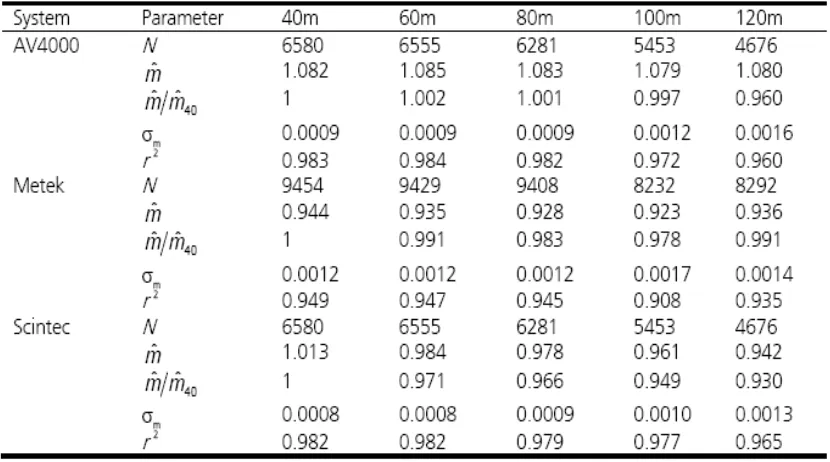
[image:29.595.101.516.456.687.2]A part of this report that is of particular interest for this thesis is the proposed calibration methods including PIE. PIE was a measurement campaign where three SODARs were operated simultaneously at the same site with comparisons to mast mounted anemometry. The aim was to use a linear model to find calibration slopes for each of the SODARs. 10 minute averages were recorded at 5 heights with varying data availability found in the different SODARs. The analysis showed that most of the uncertainty in the measurement was a result of the volume separation between the SODARs and the mast instruments. The results are shown in Table 1.3.2.
The regression slopes found are all within 10% but only some are within 5%. The R2
[image:30.595.116.481.178.420.2]correlations are generally above 0.96. Figure 1.4.1 shows the slope errors measured in the experiment for the three SODARs with respect to range gate height.
Figure 1.3.1 – Variation in regression slope with height for the measurements of a METEK (Δ), a AV4000(+) and a Scintec(O) SODAR made in the PIE from Bradley (2005).
These results show that the differences between the SODARs and the cups are between 0 and 10% and that the different SODARs give different results.
A similar inter-comparison experiment to PIE is presented in Clive (2008) and performed at Myres Hill in Scotland with a comparison between a SODAR, a LIDAR (Light Detection and Ranging) and mast mounted anemometry. The principle problem identified with the SODAR measurements is the inability to co-locate the SODAR with the mast due to the fixed echo effects SODARs are subject to. Despite a
separation distance of 300m the data between the mast and the SODAR showed good agreement. The experiment continued and the final data was revisited in Bradley (2010b) where a LIDAR was co-located with the SODAR as well as the mast in order to give a better indication of the SODARs performance. It was identified that both the SODAR and the LIDAR tended to underestimate wind speeds in comparison to the mast. The reason for this is given as the differences in measurement technique combined with the influence of the moderately complex terrain. A simple two dimensional flow model was created to explore these differences and it was found once the output of this model was taken into account the agreement between the instruments was within 2%. This study shows the most advanced use of an integrated methodology for finding the uncertainty in the SODAR measurements with the use of flow modelling and collocation of a simultaneous measurement instrument. This is the state of the art measurement approach for SODAR comparison studies. The problem with this approach is that any uncertainties in the LIDAR and mast measurements are passed on to the SODAR measurements making the best SODAR case already less certain than the LIDAR measurements and this suggests that perhaps just the LIDAR measurements at the mast position should be used.
AEP. Warmbier (2007) presents a comparison of measurements made using a mini-SODAR and cup anemometers specifically discussing the implications with regards to wind turbine power curve estimation. Using the standard linear regression R2 was
found to be 0.958. Power curves were calculated using both sets of measurements according to IEC 61400-12.
Whilst it is clear that a large volume of work has been carried out exploring the quality of SODAR data in comparison to other sensors, the results are varied and no complete calibration technique has been found using this approach. There is a risk in comparing SODARs to in-situ anemometers that an error is being introduced. Take a hypothetical case of a SODAR and a cup-anemometer measuring the exact same point in space and time, both instruments could measure exactly the same wind speed at this point however the SODAR may give a different result for the range gate containing this point due to the contribution from other parts of the volume measured. This would result in a higher error than if the SODAR result were assumed to be correct without comparison. The state of the art comparison technique consists of using CFD
modelling techniques, including those demonstrated in Mann (2000), Stangroom (2004), Bingöl (2009) and Behrens (2010b) to explain the terrain effects and the use of collocated sensors in order to find the relationship between the SODAR measurement position and that of the comparison sensors. In Boquet (2010) it was found that for one particular measurement using a WindCube LIDAR the regression slope between the wind measured by the instrument and a cup anemometer in complex terrain could be reduced from 6% to 1% through the use of CFD. Currently the use of CFD to explain wind flow in complex terrain is not fully developed although results are promising. In simple terrain the accuracy of the models is thought to be good.
1.3.4 SODAR Comparisons with Transponder Based Simulated Echoes
possible to simulate known wind speeds in a computer and use these to generate an echo signal that represents these wind speeds. In Baxter (1994 a and b) an acoustic pulse transponder (APT) system was created that contained several pre-programmed pulses to correspond to a reflection from specific heights as well as a continuous signal mode with frequency changes at known times. It has modes for both single frequency and multi frequency SODAR operation. The principle aim of this method is to
ascertain whether a SODAR can correctly measure a frequency shift and how accurate its timing is. This method was used in Fujita (1998) as part of a full quality assurance programme for air quality measurements. Figure 1.3.2 shows the flow diagram of the APT's operation. The APT itself has two variables that need to be tested in order to ensure that it provides fair testing of SODARs. These are the ability to produce known frequencies and the timing of the pulse returns, which is both the length of the pulse and the time in which it takes it to respond to the SODAR. It is stated that the system has a frequency accuracy of 1 Hz but it does not operate in 1 Hz steps due to the clock base used by the computer. Therefore SODARs tested with this system need to be operated at a matching frequency or the difference needs to be taken into account in the analysis. The system was designed to run from a small notebook and batteries meaning that it is a highly portable system which is an important design feature
Figure 1.3.2 – Flow Diagram of the Acoustic Pulse Transponder designed for USEPA quality assurance and detailed in Baxter (1994 a & b)
The early stages of a transponder system that aims to be able to find more information about the SODAR's performance is presented in Piper (2008). This transponder system features the use of signals that represent the whole measurement height and due to the signal generation methods it could theoretically represent any wind profile. Further developments in this transponder system were presented in Piper (2010) and tested in an outdoor configuration with two SODARs although the results from one highlighted that the transponder system required two further improvements before it could be a useful part of a comparison method. Part of this thesis contains results presented in these papers and continues the work on this transponder system with the aim of finding out how much information can be obtained about the operation of a SODAR through the use of a transponder containing simulated wind profiles. It is unlikely that a transponder system of this type can explain all of the uncertainty in a SODAR measurement so further alternatives to conventional SODAR-mast
1.3.5 Methods to Measure Contributing Aspects of a SODAR's Acoustic Beam Pattern
Two important aspects of SODAR measurements are defined by the SODAR's acoustic behaviour. These need to be known in order to make accurate wind speed estimations and they are influenced by the physical set-up of the SODAR including the changes caused by any baffles employed by the SODAR.
The width and shape of the measurement beam dictate the volume sampled by the SODAR and how this sampling is weighted. Measurements of the acoustic beam shape can be performed in anechoic chambers using the same approach applied to directivity measurements of Hi-Fi loudspeakers by measuring the sound pressure level at many angles in relation to the centre of the sound source. This could be performed by either measuring the whole SODAR array or measuring a single element and creating a model to find the complete directivity of the array. This is often done in SODAR design. Danilov (1992, 1994) presents a method for measuring SODAR calibration parameters in a normal sized anechoic chamber for a single horn and focussing dish SODAR measuring the sound producing element of the SODAR. This method is related to measurements of the temperature structure parameter, CT2, and not wind speed but it is of interest here since measurement of the SODAR directivity pattern is part of the procedure. Measurements of the output efficiency and input efficiency of the SODAR transducer are made and then the directivity of the horn is measured and compared to a model. The agreement between the model and
measurements are good and therefore this type of directivity model is thought to be reliable for modelling SODAR behaviour. Acoustic measurements of the SODAR directivity only allow for measurement of beam tilt angles if the whole array is measured requiring a very large space.
5% errors in the wind speed estimation. A technique is presented in Bradley (2010) for measuring the effective beam tilt angle through a level perturbation. Measurements of the wind speed are made using a SODAR fixed to a tilting mechanism. If the effective tilt angle is assumed to be unknown the introduction of a physical tilt of the whole SODAR introduces a known angle. By performing wind speed measurements with the SODAR physically tilted at two or more significantly different physical angles
analysis can be performed to to derive the effective beam tilt angle that the SODAR array is using. This method assumes a horizontally stratified flow and a constant wind speed between measurements and therefore several measurements at each tilt angle are required spread over the whole measurement period to find a reliable estimation of the tilt angle. Results from measurements made with an AeroVironment 4000 SODAR are presented and it was found that the the measured mean tilt angle was within 0.2º of the tilt angle calculated from the SODAR array geometry. This method makes no
assumptions about the SODAR and only requires a tilt mechanism and a short measurement time. It does not give any information about the beam width of the SODAR. This method will be tested and compared to other methods of measuring beam tilt angles in Chapter 4 of this thesis.
Whilst it is possible to measure the acoustic qualities of individual sound sources from within a SODAR relatively easily knowledge of how baffles alter the behaviour of SODARs is needed to give a true picture of the directivity pattern and tilt angles of a SODAR. Werkhoven (1997) investigates the use of Kirchoff integral
1.3.6 Summary
Various methods for obtaining the acoustic qualities of a SODAR have been performed but without a complete approach that is suitable for wind energy SODAR measurements. One of the aims of this thesis is to examine the possible approaches for measuring the beam shape and tilt angle in order to find an approach that can be used to reduce the uncertainty of the SODAR measurements.
1.4 Overview of the Acoustic Operation of SODARs
Mono-static SODARs operate by emitting pulses of sound in to the atmosphere and measuring the backscattered signal. The pulse is sinusoidal and it can be written as in the form of Equation 1.4.1 where A(t) is the amplitude envelope applied by the SODAR to form the pulse and D(θ) is the beam pattern of the SODAR transmitter, ω
is the angular frequency of the pulse, t is time, k is the wave number and r is the distance the pulse has travelled.
yt=AtD. e−jt−kr
(Equation 1.4.1)
The beam pattern of the SODAR is either formed from an array of loudspeakers or a single loudspeaker and a focusing dish. Each SODAR type will have a different beam pattern but all are based on first order Bessel functions of the form shown in Equation 1.4.2 where a is the radius of the loudspeaker.
D=2J1kasin
kasin (Equation 1.4.2)
Figure 1.4.1 – Amplitude Vs Angle Function, ka.sin(θ), of a First Order Bessel Function
The pulses emitted by the SODAR travel spherically away from the SODAR array and continue to travel until all the energy is dissipated through absorption and scattering. Energy which is scattered at 180 degrees is received by the SODAR as backscatter. Therefore the atmosphere can be thought of as a space containing many partial reflectors which reflect some energy back towards the SODAR. Each of these reflections has spherical wave behaviour but as the SODAR only appears on a small portion of the arc, demonstrated in Figure 1.4.2, the behaviour of the sound recorded by the SODAR can be considered to be approximately plane.
Figure 1.4.2 – Wave Front Shape of a SODAR Reflection
The energy received by the SODAR at a single point in time is a spatial average over a volume which has a weighting function formed from the beam pattern of the SODAR and the amplitude envelope applied in the range gate extraction part of the SODARs
0 2 4 6 8 10 12
-0.2 0 0.2 0.4 0.6 0.8
ka.sin(θ)
A
m
p
li
tu
d
e
(u
n
it
processing. A range gate is a section of the recorded back scatter that corresponds to a section of the height range. It is defined by the expected time it will take for sound to return from the lower and upper limits of the range gate. In the SODAR processing an amplitude window is applied that corresponds to these time limits. This means that most of the energy received by the SODAR is from within a cone with a width of between 10 and 15 degrees depending on the frequency used, the shape of the
SODAR's beam pattern and the envelope of the range gate. Different SODARs employ different range gate envelopes and have differing beam patterns, although most are similar, resulting in the effective volume of the atmosphere measured by each SODAR not being the same . This will be explored further in Chapter 2 where the directivity of different shaped speaker arrays will be modelled and the effects on the SODAR measurement explained.
The sources of reflection for mono-static SODARs are temperature fluctuations that have a size comparable to half a wavelength. The fluctuations travel with a
velocity that is the sum of the mean wind speed and local turbulence. Sound which is reflected by a moving medium is shifted in frequency according to the Doppler Effect. Therefore sound received by the SODAR will have a frequency content which is directly related to the wind speed at the point of reflection. As the sound received by the SODAR at a single point in time is a spatial average of many reflections, the recorded backscatter is a signal which has a frequency peak which corresponds to the mean wind speed in the volume but with spectral width determined by the level of variation over the measurement volume. The magnitude of the temperature
fluctuations will also vary and therefore the strength of the return will change accordingly.
The amplitude of SODAR echoes decay in time due to the effects of spherical spreading and atmospheric absorption. The amount of decay is dependent on the
from Salomons (2001). Equation 1.4.3 describes the amplitude envelope of a SODAR echo where σs is the scattering cross section, c is the speed of sound, τ is the pulse
duration, α is the absorption of air and z is the height of the echo source. This envelope scales with the power transmitted by the SODAR.
Et=sc
2
e−2z
z2 (Equation 1.4.3)
The scattering cross section is described by Equation 1.4.4. where λ is the wavelength of the sound, C2
T is the temperature structure function and T is the lapse rate corrected
temperature based on the ground temperature, TG. Typical values of C2T are close to
10-4 .
s=6e−4
−1/3CT
2
T2 (Equation 1.4.4)
The absorption of sound in air is described in the empirical formula shown in Equation 1.4.5 where f is the frequency of the sound in Hz, t is the lapse rate (L) corrected
temperature T divided by the ideal maximum temperature, 293.15 K, P is the
atmospheric pressure given by Equation 1.4.6, fn and fo are relaxation frequencies for
nitrogen and oxygen respectively and are calculated using Equations 1.4.7 and 1.4.8 respectively, g is the acceleration due to the force of gravity, which is approximately 9.81 ms-2, and R is the specific gas constant, which is 287 Jkg −1 K−1 for air. H is humidity and it is calculated using Equation 1.4.9 where RH is relative humidity in percent.
=8.686 f2t1/2
1.84e
−11
P
0.1068e−3352/T
fnf2
/fn
0.01275e−2239.1/T
fof2
/fo t
−3
(Equation 1.4.5)
P= T
TG
g
f o=P2440400H 0.02H
0.391H (Equation 1.4.7)
fn= P
t1/29280He
−4.17f−3−1
(Equation 1.4.8)
H=RH
P 10
4.615−6.8346TG
T
1.261
(Equation 1.4.9)
From the above set of equations the expected time-amplitude envelope of a SODAR echo can be predicted for a given set of atmospheric variables. The effects of the different variables contained within the envelope equations are explored at length in Harris (1966), Evans (1972) and Bass (1972 and 1995).
A SODAR echo has a frequency shift according to the mean wind speed in the direction of the beam, a spectral broadening due to the velocity and reflection strength variation across the measurement volume, amplitude fluctuations which follow
variation in the magnitude of temperature fluctuations and a time-amplitude envelope which decays in a partly exponential manner. The echo arrives at the SODAR from the direction in which the SODAR emitted the corresponding pulse and it has
approximately plane wave behaviour. The SODAR itself contains a signal chain performing a combination of filtering, amplification and Fourier analysis in order to calculate a wind speed estimate. The aspects of this chain vary between different SODARs but are all aiming to find a reliable estimate of the wind speed. The different methods are discussed at length in various texts including the WISE report, detailed in the following section, and Bradley (2008) and some investigation of some aspects of this process that have an obvious and quantifiable effect on the wind speed estimation are discussed in Chapter 2.
1.5 Statement of the Aims of This Thesis
independent measurement methods in combination with established ones to mono-static SODARs and exploring the statistical significance of SODAR measurements with a focus on the measurements meaning to the wind incident or turbines.
Conventionally the quality of SODAR measurements are determined by making comparisons with measurements made by mast mounted anemometers. This has some inherent problems due to the differences in the actual measurement which is being carried out and therefore such comparisons are limited to a coarse indication of
measurement accuracy and highlighting strong mismatches rather than ensuring actual measurement accuracy. Many previous studies have been carried out using
comparisons to mast mounted instruments with some studies suggesting rules for interpreting the differences between the two measurements. Some studies have
suggested alternative methods to this approach although a comprehensive method has yet to be created. By review of this past work and through the development of a mast independent calibration techniques it is hoped that mono-static SODAR accuracy can be verified and quantified. This work should also increase understanding of the
processes which affect mono-static SODAR measurements and improve acceptance of mono-static SODAR measurements in the wind energy field.
The principle research questions are as follows:
i) Can the quality of SODAR measurements be improved and uncertainty reduced through theoretical analysis of the acoustic behaviour of SODARs?
ii) Can a transponder system be created that goes further than a simple diagnostic test to find information about the SODAR's operation and offer the possibility of direct comparison between the measurements of different SODARs with the ability to test in the field?
shape and tilt angle?
iv) Can these aspects be combined into a unified approach to
improve SODAR measurement certainty and therefore increase the usefulness of SODAR measurements for the wind industry?
1.5.1 The UpWind Project
This thesis is written as part of the UpWind Project. The UpWind project is a European Government sponsored project which aims to increase the size of wind turbines for both on shore and off shore use by solving the design problems involved in up scaling turbine sizes to 8-10 MW. The work package it is part of is an
examination of the use remote sensing techniques, focussed on LIDAR and SODAR, as potential replacements for mast mounted measurements. Specifically this thesis aims to form the SODAR part of Section 2 of the work package although there will be some overlap with Section 1. Section 2 is an investigation into traceable calibration techniques for remote sensing instruments and Section 1 is an in depth description of the measurement process. It is debatable whether a calibration is actually what is required for SODAR measurements to be useful for wind energy and it is thought that a verification is a more appropriate term for what can be applied although this is a semantic debate. The effect on the measurement made by a SODAR of a certain physical set-up and operational parameters is crucial to reducing uncertainty. The only part of the operation that offers the opportunity for a true calibration beyond individual component testing is the beam tilt angle and some effort is given to finding the best methods for quantifying this.
Within the UpWind work package investigation into several aspects of the use of remote sensing in wind energy has been and continues to be performed. This
Foussekis (2010). This work is all carried out using LIDAR instruments and necessitates the work in Gómez (2010c) and Hill (2010a) on finding methods to correct or filter for cloud and fog. LIDARs are also required to have traceable calibration methods. Work investigating this is detailed in Hill (2010b). How this is related to SODAR calibration will be discussed in Chapter 5.
1.6 Outline of Methods to Explore SODAR Measurement Uncertainty
The methods explored in this thesis are split into three parts following the first three research questions: theoretical analysis, transponder measurements and
directivity measurements. Each adds a different aspect to improving the uncertainty and interpretation of SODAR measurements. The theoretical analysis uses acoustic theory to explore the behaviour of different common SODAR configurations focussing predominately on the effects of array geometry. The transponder measurements use a transponder system that has been developed for this thesis with some basis in the work carried out in Baxter (1994). Directivity measurements are carried out using several different methods with comparisons between these methods and recommendations of how to perform further measurements. These aspects of a SODAR's operation can lead to the largest uncertainties in the wind speed estimation and therefore it is of great importance to find a method that can measure these details to a high resolution. These separate aspects are then discussed and combined to answer the 4th
research question.
1.7 Summary
and carried out in the Myres Hill comparison experiment. These methods mean the best result achievable is that the SODAR has the uncertainty of the reference sensor.
Methods to reduce SODAR uncertainty without making comparisons to other sensors are required. A simple transponder system is one alternative although
transponders have only previously been used as a diagnostic tool. Methods to
2. Theoretical Comparison of Known Differences Between
SODARs
2.1 Introduction
When comparing measurements from different SODARs, the differences in the way the SODARs operate and differences in their location and set-up need to be taken into account. If all aspects of the operation of the SODAR are known then this can be done theoretically. Taking the hypothetical case of two SODARs situated in exactly the same place at the same time it is possible to examine the effect of the various
parameters on the measurements made since the physics of sound travelling through the atmosphere will be identical in each case. Both physical and processing parameters can be explored in this way.
The physical parameters of a SODAR are related to the directivity pattern, which can be modelled using a far field model of the radiation from two dimensional speaker arrays. The width of the central lobe alters the effective volume from which reflections are recorded. The directivity pattern in combination with the baffle shape alter the influence of fixed echoes on the SODAR measurement. The angles at which the SODAR beams are tilted affect the resolution, the volume separation between the beams and the susceptibility to errors caused by a non level set-up, which can either be a result of incorrect physical set-up or a consistent phase problem across a speaker array.
beam tilt angle does not match the beam tilt angle that is used in the processing it is preferable to consider this a physical parameter.
This chapter will examine each of these issues in turn and quantification of the effects of the possible options in each case will be given. Some of the topics described have been covered in depth in other works so are only outlined here with references for the sake of providing a full description.
2.2 Far-field Model of Sound Radiation from 2D Speaker Arrays
Analytical models for the behaviour of sound sources are well established in text books such as Kinsler (2000). The underlying principle is that any sound source can be modelled as an infinite number of point sources. A point source is a theoretical source which can be described as an infinitesimally small pulsating sphere radiating energy equally in all directions. An equation exists that describes the directional behaviour of a circular source such as a speaker as shown in Equation 2.2.1 where
Hs(θ) is the angular dependent amplitude function for the source, J1 is a Bessel
function of the first kind, k is the wave number and a is the radius of the source.
Hs=2J1kasin
kasin (Equation 2.2.1)
An example of this function is shown in Figure 2.2.1 for a ka value of 6.65 based on a frequency of 4500Hz and a source radius of 8cm. The assumption made in this
Figure 2.2.1 – Directivity pattern, Hs, for a single circular source.
Expressions exist for the combination of a column of several separate monopole
sources that emit either the same sound, Equation 2.2.2, or sounds with a known phase relationship, Equation 2.2.3, where Hc(θ) is the angular dependent amplitude function
for the combination of point sources in a column, N is the number of sources in the column, d is the separation between the centre of each source and θO is the phase shift.
Hc=
1 N
sin[N
2 kdsin] sin[1/2kdsin]
(Equation 2.2.2)
Hc=
1 N
sin[N
2 kdsin−sin0] sin[1/2kdsin−sin0]
(Equation 2.2.3)
These equations give the directivity pattern generated by a column made up of monopole sources. Figure 2.2.2 shows examples of these functions.
-80 -60 -40 -20 0 20 40 60 80 -60
-50 -40 -30 -20 -10 0
Angle (°)
N
or
m
al
iz
ed
A
m
pl
itu
de
(
d
B
/d
B max