Parametric Study of Flow Characteristics of Butterfly Valve using CFD

(1)

International Journal of Emerging Technology and Advanced Engineering

Website: www.ijetae.com (ISSN 2250-2459,ISO 9001:2008 Certified Journal, Volume 5, Issue 11, November 2015)

142

Parametric Study of Flow Characteristics of Butterfly Valve

using CFD

Naveen Kumar C

1

, V Seshadri

2

, Yogesh Kumar K J

3 1_{M.Tech Student, Thermal Power Engineering, MIT – Mysore, India}

2_{Professor (Emeritus),}3_{Assistant Professor, Department of Mechanical Engineering, MIT-Mysore, India} Abstract— Butterfly valve is a flow control device, which is

used to regulate the fluid flowing through a piping system. Analysis and optimization are of special importance in the design and usage of butterfly valves. A proper selection of a Butterfly valve would require the knowledge of its characteristics and robustness. Normally this information used to be obtained from experimental tests. However the tremendous improvements in the computational methodology in recent times, has enabled the analysis of Butterfly valves using available commercial software. This paper deals with CFD analysis to find the effect of Reynolds number and the various valve openings on the characteristics of a traditional butterfly valve. The pressure loss coefficient has been evaluated at various operating conditions of a Butterfly valve. Further the permanent pressure loss coefficient has also been computed and its dependence has been analysed so that the recovery of pressure after passage through valve could be quantitatively understood.

Keywords—Butterfly Valve, Pressure loss Coefficient, Permanent Pressure loss Coefficient, Drag force, Disc shape.

I. INTRODUCTION

A butterfly valve is a device that controls the flow of gas or liquid to control the internal flow of both compressible and incompressible fluids in piping systems. They are commonly used in applications where the pressure drops required is relatively low. It consists of a metal disc with its pivot axis at right angles to the direction of flow in the pipe. The rotary movement offered by the valve stem is about 90 degrees. So, these valves are also called as quarter turn valves. Characterizing a valve‘s performance factors, such as pressure drop, flow coefficient and loss coefficient, is necessary for fluid system designers to account for system requirements to properly operate the valve and prevent damage. How a butterfly valve will perform, while in operation at different opening angles and under different types of flow, is critical information for engineers planning and installing piping systems involving the valve. Performance factors common to a butterfly valve include the pressure drop, flow coefficient and loss coefficient.

While these values can usually be obtained experimentally, it is often not feasible or possible to calculate the performance factors of butterfly valves. Another method wherein butterfly valve performance factors can be obtained is by using Computational Fluid Dynamics (CFD) software to simulate the physics of fluid flow in a piping system around a butterfly valve.

Pressure loss coefficient ( )

The value of the pressure loss coefficient (ζ) is calculated by considering the difference in pressure between two locations, one at upstream and other at downstream of the pipe line. Thus, ζ is defined as,

Where, ΔP=Pressure drop across the valve in Pas

ρ = Density in kg/m3

v = velocity in m/sec,

ζ = Pressure loss coefficient.

The introduction of the valve disc introduces certain permanent pressure loss in the duct. In order to evaluate its magnitude, the pressure loss in the duct with and without valve is computed at identical flow conditions. Thus the following pressure drops namely, ΔP1, ΔP2.are calculated.

∆P1 = Pressure drop between inlet and outlet of the duct

with the valve disc.

∆P2 = Pressure drop between inlet and outlet of the duct

without valve disc.

Both ∆P1 and ∆P2 are computed in the identical flow

conditions and obviously

∆P1 > ∆P2.

Thus, permanent pressure loss is defined as,

(2)

International Journal of Emerging Technology and Advanced Engineering

143

Permanent pressure loss coefficient is defined as,

Also,

This parameter represents the extent of energy loss in the duct due to the introduction of the valve. It has been evaluated for all the cases studied.

II. BACKGROUND

The behaviour of a Butterfly valve in flow field has been studied by several researchers. Some of them are discussed below.

Ghaleb Ibrahim et.al [1], focussed on the visualization of flow characteristics around the Butterfly valve. For this purpose, they have used commercial FLUENT software. They concluded that the flow velocity remains constant till it reaches valve and start to change in the downstream. Vortices are generated in the downstream of the flow path. Turbulence appears at the edges of the valve. At partial loads the pressure losses are more.

Takeyoshi Kimura et.al [2], made an attempt to investigate the characteristics of Butterfly vales by conducting an experiment. Finally they concluded that the loss coefficient at partial openings near the middle value does not depend on the shape of the valve. But at fully opened condition, there is a difference in loss coefficient. The valves with sharp leading edges show more pressure loss because of separation of flow.

A.D.Henderson et.al [3], studied flow through butterfly valve as a safety device in hydroelectric `power scheme. ANSYS designer modeller was used for the analysis. They verified the factors affecting the results such as Reynolds number and unsteady flow. They finally concluded that flow becomes unsteady over a range of valve opening angles. CFD gives better results when we give more representative conditions of the actual flow field.

Xue guan Song et.al [4], Concentrated on the flow characteristics around the Butterfly valve. Simulations were done to study the variation of flow coefficient, torque coefficient for different valve opening angles with uniform inlet velocity. The turbulent model used was the k-ɛ model.

So, they finally concluded that at 20° and below opening angles experimental data did not match very well with the simulated values because at these regions k-ɛ model didn‘t give accurate result and CFX code is very sensitive near fully closed valve opening angles.

B.Prema et.al [5], carried out simulations with a 3D, steady, incompressible turbulent k-ɛ model. Two different geometries of the valve disc were modeled namely, Baseline design (Valve with convex profile and a stem in one side and a flat profile on the other side) and Optimized design (Convex profile one side and concave profile on the other side and the stem removed by pivoting the disc at the ends). Optimized design reduces the manufacturing cost and weight of the valve and also improves the flow field.

S Y.Jeon et.al [6], made an attempt to do a comparative study of two types of Butter fly valves (single disc and Double disc). Experimental values were compared with the numerical predictions. The values of flow coefficient against valve lift and loss coefficient against valve lift were plotted for both single and double disc cases. The experimental and numerical results matched reasonably well. However the flow pattern of the double disc valve showed complex structure when compared with the single disc.

Mehmet Sandalci et.al [7] has conducted experiments on Butterfly valves with two different sizes (DN65 and DN80) at different velocities (2, 3, and 4m/s) at different valve opening angles (0 to 40 degrees). They calculated flow area percentages for different openings. Using experimental data, loss coefficient, flow coefficients were calculated. Correlations were made to get loss and flow coefficients in terms of percentage flow area. The conclusions made were Pressure loss coefficient was independent of velocity but depends on the valve size at lower opening angles. Flow coefficient was independent of velocity but depends on the valve size.

A.Dawy et.al [8] used ANSYS FLUENT code and the standard k-ɛ model to evaluate the performance factor such as flow coefficient for different valve openings. The results showed good agreement with experimental data. They concluded that CFD provides a means of gaining valuable insight into the flow field of the valve, where complex fluid structure and velocity profile recovery can be observed and studied.

(3)

International Journal of Emerging Technology and Advanced Engineering

144

They observed that the average pressure is maximum when the opening angle is 10 degrees. And total force on the disc is maximum when the opening angle is 40 degrees. By changing the disc shape two different zero torque angles could be seen, which means that the valve will be self-operating at these angles.

Several studies using CFD to analyse the flow through Butterfly valves are reported in the literature. However, all the geometrical parameters as well as flow parameters have not been covered over the entire range. Thus, very little is known about the performance of Butterfly valve at low Reynolds numbers. Further, the variation of Permanent pressure loss coefficient as well as the dependence of pressure distribution on the valve disc under different operating conditions is not fully understood. Hence the present study is aimed at understanding some of these aspects

III. MATHEMATICAL MODEL AND CFDMETHODOLOGY

The analysis of a Butterfly valve practically is a time consuming and also a complicated process because of its constructional constraints. Nowadays CFD is being used to analyse these complicated problems to save money and time.

The equations like conservation of mass, conservation of momentum and conservation of energy are being used by the CFD code Fluent.

2.1 Conservation of mass equation:

For two dimensional incompressible and compressible fluid flows.

2.2 Conservation of momentum equation:

For two dimensional steady flows:

( )

Where,

p = the static pressure. g = Gravitational body force.

In turbulent flow, these equations are time averaged to yield RANS equations which will necessitate turbulence modeling.

In the present study k-ɛ model is used for the analysis. Where k is turbulent kinetic energy and ɛ is the rate of viscous dissipation the model equations are given below.

[ ] [ ]+2 - ρɛ

[ ] [ ]+ 2 -

Where eddy viscosity is defined as follows,

= ρ , Here is a dimensionless constant.

The k-ɛ model is the one which is most widely used in many industries because of its simple operating procedures (only requires initial and boundary conditions).The above equations are solved numerically using finite volume method.

IV. VALIDATION OF CFDMETHODOLOGY

[image:3.612.330.558.437.664.2]

The developing flow through a circular straight pipe for turbulent flow is considered for validation. The dimensions and the Boundary conditions applied are as shown in below table.

Table .1

The Dimensions of the Geometry used for the Validation

Parameters Dimensions

Pipe Length (m) 6

Pipe Height (m) 0.06

Inlet velocity (m/s) 1

Viscosity (kg/m-s) 0.001003

Reynolds No 59821

[image:3.612.46.254.498.666.2]

Turbulent model used k-ɛ standard

(4)

International Journal of Emerging Technology and Advanced Engineering

[image:4.612.322.560.112.232.2]

145

Fig. 2 Grid used for pipe flow analysis.

An axi-symmetric circular pipe model (Fig.1) of length 6m and height of 0.06m has been made using ANSYS software. A velocity of 1 m/s at inlet, ambient pressure at outlet and No-slip condition at wall were used as boundary conditions for the flow domain in the simulation process. The convergence criterion is 10-7. Pressure drop for theoretical analysis was extracted from the software (at 3 m and 4.8 m from inlet). The results are tabulated in Table.2. The values in the table show that the theoretical and CFD results are fairly close to each other. Further the fully developed values of the velocity at the axis of the pipe are compared with the standard values in Table2. It is to be noted that the values quoted in the literature for the ratio Umax / Uavg vary significantly in different sources. An

average value of 1.2 is chosen for this ratio based on several researches. This value compares very favourably with the computed values. The entry length in the pipe line is defined as the distance from the inlet at which the axial velocity reaches 99% of the fully developed value. In turbulent flow, the entry length is usually taken as 50D.It is observed from the Table 2 that the computed values of the entry length are in good agreement with the above criteria. Hence the CFD methodology used in the study is validated. For this particular flow k-ɛ standard model is adequate.

According to the mesh convergence study the quadrilateral elements (Fig.2) around 185000 yields better results. And different turbulence models have been studied and the study revealed that K-ɛ standard model gave the best trend.

[image:4.612.67.274.137.217.2]

The results obtained from the above validated problem are tabulated below.

Table .2

Theoretical and CFD values for the Validation Problem with k-ɛ standard model

Parameters Theoretical results CFD results

Pressure Drop(Pas)

(∆P) 313 293

Entry length(m) 3 2.5

Umax / Uavg 1.20 1.18

1

Fig.3 Pressure and Velocity plots

On the basis of above comparisons, the CFD methodology can be taken as validated. Hence in all the further analyses similar discretization is used and k-ɛ model was chosen when the flow is turbulent.

Flow through an actual Butterfly valve at various valve openings is in fact highly complex. The flow is 3D and at partial openings, flow gets separated at the valve disc and the regions of recirculation are observed. Thus, the analysis of flow will require large amount of computing power and the computing system having large memory. However at present, the computing facilities available in the institution are modest and hence the geometry has been idealized so that the analysis can be carried out. Hence for the analysis, the fluid is assumed to be incompressible and Newtonian. The duct is assumed to be 2D and the flow is considered to be steady. Nevertheless the flow can be either laminar or turbulent depending on Reynolds number.

V. 2DMODELING OF FLOW THROUGH BUTTERFLY VALVE

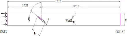
In order to model the flow through Butterfly valve, the disc is placed inside a two dimensional duct with upstream and downstream straight lengths. It is important to have these straight lengths sufficiently larger so that the flow around the valve disc is not affected by the boundary conditions at the inlet and outlet of the duct. Flow domain considered is as shown in the Fig 4.It consists of a two dimensional duct having a total length of 500mm and the width of the channel is 40mm. thus the total length of the domain is 12.5H, where ‗H‘ is the width of the duct. The valve disc is placed at a distance of 3.75H from the inlet of the duct.

[image:4.612.335.555.616.683.2]

(5)

International Journal of Emerging Technology and Advanced Engineering

146

Discretization

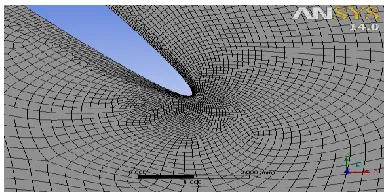
[image:5.612.71.267.227.331.2]

The discretization of the flow domain is carried out with 2D quadrilateral elements. A structured mesh has chosen for the analysis. The region around the valve disc has been meshed with a very fine mesh structure, so that the flow details are captured accurately. A sample mesh around the valve disc is as shown in Figs 5 and Fig 6

Fig. 5 Sample Mesh around the Valve Disc.

Fig. 6 Details of the Mesh Around The Edges Of The Valve Disc.

It is observed that regions around the valve are meshed with very fine mesh, as the velocity gradients in this region are expected to be high. The number of elements used for discretization is in the range of 1x105 to 3x105. It is also observed from the figure that the edges of the disc are rounded to reduce the separation losses.

Boundary Conditions

The boundary conditions used are the following. (See Fig. 4)

 At the inlet face - Velocity inlet is specified. The velocity of the fluid is taken as uniform across the width of the duct.

 The duct walls and the surface of the valve disc are specified with no-slip wall condition.

 At the outlet of the duct - Pressure outlet condition with gauge pressure being zero is specified.

Extensive analyses have been made by varying different geometrical and flow parameters. For each case, the mesh is generated separately whenever needed. In particular, the following parameters have been varied.

 Analyses have been made for eight different openings of the valve disc in the range of 30° to 90°.For each opening separate discretization is done.

 The Reynolds number of the flow is varied from 1 to 104, thus covering both laminar and turbulent regions. Reynolds number is defined as,

Re =

Where ρ = Density of the fluid in Kg / m3. v = Velocity in m / sec. H = width of the duct in m.

μ = Viscosity of the fluid in Pa-s

The values of ρ, v, μ are chosen appropriately to obtain the desired Re, In order to keep pressure differentials with in a range, the velocity is assumed to be in the range of 0.5 to 2 m/sec. Thus the value of viscosity is varied to analyse the effect of Re.

In both the above analyses, the wall is assumed as smooth and the default value of turbulent intensity is specified at the inlet.

Analysis of the Numerical Results

The computed pressure and velocity field have been further proceeded to extract various practical information. Velocity and pressure plots are plotted to get an insight into the flow around the valve. Further, velocity vector plots gave details about the flow pattern in the downstream region of the valve.

The values of the pressure loss coefficient (ζ) and permanent pressure loss coefficient (ζp) are also computed

in each case. These coefficients have already been defined in the earlier section.

The pressure distribution on the face of the disc as well as the drag force is also calculated from the computed results.

Selection of Turbulent Model

[image:5.612.71.265.359.456.2]

(6)

International Journal of Emerging Technology and Advanced Engineering

147

The default values for the constants in each model given in the software were used for these computations. Based on this analysis, it was observed that k-ε standard model gives the most accurate trends in the computational results. Hence this model has been chosen for the study. The computations have been carried out by specifying the convergence criteria 10-7for residuals. Each computational run approximately took 8 to 10 hours for convergence on a machine with the following specifications.

Specification

Intel(R) Core(TM)

i3 - 2100 CPU @ 3.10GHz

3.09GHz.2.99GB of RAM

VI. RESULTS AND DISCUSSION

In standard literature like ASME, JIS etc., valve coefficient (Cv) of a valve in a duct signifies the mobility of

the flow for the corresponding opening of the valve. Cv is

defined as,

CV =

Where, Q is Flow rate in USgpm. G is specific gravity of the fluid and

∆P is the pressure drop across the valve in Pas. However in the present study, since the geometry is 2D the pressure loss coefficient ζ is calculated. Pressure loss coefficient (ζ) is the dimensionless pressure loss across the valve. This means that ζ is inversely proportional to Cv2.

Computations have been made for various opening angles of the valve. At each opening, Re of the flow is varied in the range of 1 to 104.For all computations the density and the velocity is taken as 1000 kg/m3 and 2 m/s respectively. The desired Re is obtained by choosing the appropriate value of viscosity (μ). When the flow is turbulent K-ɛ model is used. And the convergence criteria are taken as 10-7. The wall of the pipe and the valve is assumed as smooth. And inlet turbulent intensity has taken as default.

The results obtained from the various parametric studies are individually discussed in the following section.

Effect of Reynolds Number

The effect of Reynolds number on the characteristics of the valve has been systematically studied. For this purpose an elliptical disc of 38mm diameter and 3mm thickness is chosen. Computations have been made at two valve openings namely, 30° and 60°.Calculations have been made at six Re namely 1 , 10, 100, 1000 and 79760.At each Re the value of ζ and ζp are calculated.

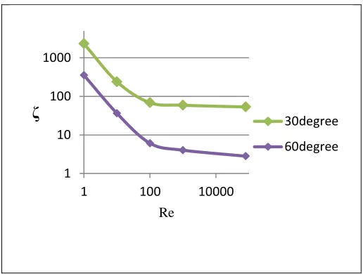
[image:6.612.315.573.370.565.2]

The relation between Pressure loss coefficient and Reynolds number is shown in Fig 7. In the range of Re 1 to 103 the magnitude of ζ reduces monotonically. The computed values are tabulated in Table 3. It is observed that at both valve openings, the value of ζ remains more or less constant at higher Re (turbulent regime). Thus it can be concluded that in turbulent flow the ζ remains fairly constant. The increase in the value of ζ with decreasing Re can be attributed to higher viscous losses at lower Re. It is also observed that at any given Re the values of ζ at 30° is much higher than those at 60° opening. This is obviously due to the higher blockage at smaller opening.

Fig. 7 Variation of ζ with Different Re for Disc Inclined at 30° and 60° (v = 2 m/s, Elliptical Disc, Disc Thickness = 3mm, Disc height =

38mm)

1 10 100 1000

1 100 10000

ζ

Re

30degree

(7)

International Journal of Emerging Technology and Advanced Engineering

148

Fig. 8 Variation of ζp with Different Re for Disc Inclined at 30° and 60° (v = 2 m/sec, Elliptical Disc Shape, Disc Thickness = 3mm, Disc

height = 38mm)

The variation in Permanent pressure loss coefficient (ζp)

with Re is shown in Fig 8. And the values are tabulated in Table 3. It is observed that the variation in ζp is similar to

that of ζ. It is observed from the tabulated values that the value of ζp is always lower than ζ at any given flow

conditions and valve openings, this is due to partial recovery of pressure after the passage through the valve. It is also observed that the recovery is higher in the case of larger valve opening. Further in laminar flow the pressure recovery is somewhat higher.

Table 3

ζ and ζp Values with Different Re for Disc Inclined at 30° and 60°

Re ζ for 30° ζ for 60° ζp for 30° ζp for 60°

1 2325.18 354.69 2235.16 264.69

10 240.22 36.35 231.22 27.35

100 68.71 6.09 67.68 5.07

1000 59.071 4.02 58.83 3.78

[image:7.612.319.560.99.695.2]

79760 53.18 2.81 53.10 2.74 Figs 9 and 10 show the pressure and velocity contours at valve opening of 30°at Re = 10 and 79760. The corresponding plots at valve opening of 60° are shown in Figs 11 and 12. It is observed that variation in pressure and velocity fields show marked difference in laminar and turbulent flows. In turbulent flows the pressure and velocity fields are much more non-uniform.

[image:7.612.45.292.118.313.2]

Fig. 9Pressure and Velocity Contours for Disc Inclined at 30°with Re=10

Fig. 10 Pressure and Velocity Contours for Disc Inclined at 30° with Re=79760

Fig. 11 Pressure and Velocity Contours for Disc Iinclined with 60° at Re = 10

[image:7.612.41.296.493.569.2]

Fig. 12 Pressure and Velocity Contours for Disc Inclined at 60° with Re = 79760

Fig. 13.Velocity Vector Plots for Disc Inclined at 30° with Re = 10 and 79760

Fig. 14. Velocity Vector Plots for Disc Inclined at 60°

with Re = 10 and 79760

1 10 100 1000

1 1000

ζ

_p

Re

30degree

(8)

International Journal of Emerging Technology and Advanced Engineering

149

Fig. 13 and 14 show the velocity vector plots at two valve openings of 30° and 60° for two Re, one in laminar and other in turbulent regime. The flow structure in the separated region behind the disc can be clearly seen from these plots. In laminar flow the wake region is much smaller as compared to turbulent flow. Further at smaller valve opening recirculation zones are somewhat larger

Effect of Valve Opening(θ)

The effect of valve opening on the characteristics of the valve has been studied. For this purpose an elliptical disc of 38mm diameter and 2mm thickness is chosen. Computations have been made at eight valve openings namely, 30°,40°, 50°, 55°, 60°, 70°, 80° and 90°.Calculations have been made at Re = 79760.At each valve openings ζ and ζp are calculated.

Fig.15. Variation of ζ and ζp with Various Valve Opening angles. (Re = 79760, v = 2 m/s, Elliptical Disc Shape, Disc Thickness = 2mm,

Disc height = 38mm).

[image:8.612.379.498.127.296.2]

The relation between Pressure loss coefficient and valve opening is shown in Fig. 15. In the range of θ = 30° to 90°, the magnitude of ζ reduces monotonically. The computed values are tabulated in Table 4. As expected the value of ζ decreases very rapidly with the increase in valve opening. This is obviously due to a reduction in the obstruction caused by the disc to the flow and the consequent decrease in the energy dissipation.

Table 4

ζ Values with Different Valve Opening Angles.

θ ζ ζp

30° 57.23 57.14

40° 20.75 20.68

50° 7.96 7.89

55° 4.94 4.87

60° 3.02 2.94

70° 1.02 0.95

80° 0.31 0.24

90° 0.12 0.05

It is also observed from the tabulated values of ζp in

Table 4 that the variation with θ is similar to that of ζ. At any given opening the value of ζp is lower than that of ζ

[image:8.612.50.287.324.477.2]

although the difference is not very large. This indicates that the pressure recovery in the downstream of the valve is not very significant.

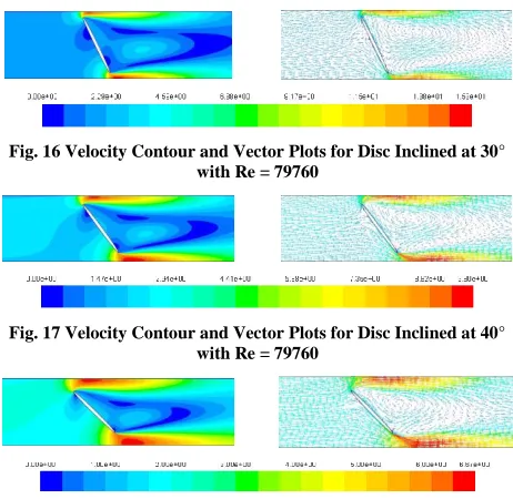
Fig. 16 Velocity Contour and Vector Plots for Disc Inclined at 30° with Re = 79760

[image:8.612.328.559.368.593.2]

(9)

International Journal of Emerging Technology and Advanced Engineering

[image:9.612.51.285.107.527.2]

150

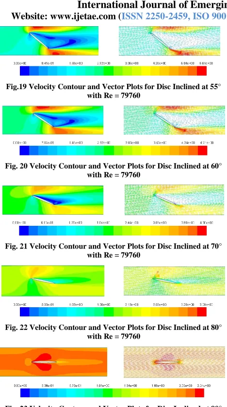
Fig.19 Velocity Contour and Vector Plots for Disc Inclined at 55° with Re = 79760

Figs 16 to 23 show the velocity contour and the corresponding velocity vectors for valve opening angles 30° to 90° that are chosen for the present study. From these Figs we can clearly observe that the range of velocities encountered in the flow domain keeps on decreasing as the valve opening increases. Thus the maximum value of velocity at θ = 30° is 15.3m/s whereas the corresponding values at θ = 50 and 80 are 6.67m/s and 3.56m/s respectively. It is also observed that the flow pattern in the wake portion of the disc undergoes drastic changes with change

VII. CONLUDING REMARKS

A validated computational methodology for analysing 2D flow through Butterfly Valve has been presented. k-ɛ turbulent model is found to be more suited for this class of flows. The pressure loss coefficient decreases rapidly as the valve opening increases from the fully shut condition. The decrease becomes more moderate as we approach fully opened condition. Reynolds number has a significant effect on the value of ζ .In the laminar flow its value is much higher and decreases rapidly with increase in Re. In the turbulent regime the variation is very minor.

This analysis has been extended to analyse the effect of various opening angles on drag force on the valve disc.The effect of variation in geometrical parameters like disc thickness, disc shape, and the size (height) of the disc on the pressure drop characteristics have also been analysed. These will be presented in future publication. Attempts are also being made to extend the analyses to 3D flows so that actual geometry of the valve as well as torque characteristics can be modelled.

REFERENCES

[1] Philip L. Skousen. Valve Hand book – Second edition – McGraw-Hill publications,1998.

[2] Ghaleb Ibrahim, Zaben Al-Otaibi, Husham M.Ahmed. ―An investigation of Butterfly valve flow characteristics using numerical technique‖. Journal of Advanced Science and Engineering Research, Kingdom of Bahrain, Vol-3, pp.151-166, 2013.

[3] Takeyoshi Kimura, Takahara Tanaka, Kayo Fujimoto, Kazuhiko Ogawa. ―Hydrodynamic Characteristics of a Butterfly Valve – Prediction of Pressure loss Characteristics‖. ISA Transactions, Japan, vol-34, pp.319-326, 1995.

[4] A.D Henderson, J.E Sargison, G.J.Walker, J Haynes. ―A Numerical Study of the Flow through a Safety Butterfly Valve in a Hydroelectric Power Scheme‖. 16th Australasian Fluid Mechanics Conference, Australia, pp.1116-1122,2007

[5] Xue guan song, Young Chul Park. ―Numerical Analysis of butterfly valve – prediction of flow coefficient and hydrodynamic torque coefficient‖t. World Congress on Engineering and Computer Science, USA, 2007.

[6] B.Prema, Sonal Bhojani, N Gopalakrishnan (2010).‖Design Optimization of Butterfly Valves using CFD‖.4th International Conference on Fluid Mechanics and Fluid Power, Chennai, India, pp.1-7, 2010.

[7] S Y Jeon, J Y Yoon, M S Shin. ―Flow Characteristics and Performance Evaluation of Butterfly Valves using Numerical Analysis‖.25th IAHR Symposium on Hydraulic Mechanism and Systems. Republic of Korea, pp.1-6, 2010.

(10)

International Journal of Emerging Technology and Advanced Engineering

151

[9] A Dawy, A Sharara, A Hassan. ―A Numerical Investigation of the

Incompressible flow Through a Butterfly Valve‖. International Journal of Emerging technology and Advanced Engineering, Egypt, Vol-3, pp.1-7, 2013.

[10] ANSYS FLUENT theory guide published by Ansys.in in April 2009.

[11] Frank.M.White, ―Fluid Mechanics‖ Seventh edition, published by Tata McGraw-Hill Publication company, Special Indian Edition 2011, 2008.