Development of new cost sensitive Bayesian network learning algorithms

DEVELOPMENT OF NEW COST-SENSITIVE

BAYESIAN NETWORK LEARNING

ALGORITHMS

Eman Bashir Nashnush

SCHOOL OF COMPUTING, SCIENCE AND ENGINEERING,

INFORMATICS RESEARCH CENTRE, COLLEGE OF SCIENCE AND

TECHNOLOGY, UNIVERSITY OF SALFORD, UK

i

TABLE of CONTENTS ... i

LIST of FIGURES ... iv

LIST of TABLES ... vi

LIST of ABBREVIATIONS and SYMBOLS ...vii

ACKNOWLEDGMENTS ... viii

LIST of PUBLICATIONS...ix

ABSTRACT ... x

Chapter 1: Introduction ... 1

1.1 Introduction ... 1

1.2 Motivation ... 3

1.3 Research aims and objectives ... 5

1.4 Research questions ... 6

1.5 Research methodology ... 7

1.6 Thesis organisation ... 9

Chapter 2: Background on Bayesian Networks ... 11

2.1 Data Classification ... 11

2.2 Overview of Bayesian networks ... 13

2.3 Principles of Bayesian networks ... 15

2.3.1 Definitions from probability theory ... 15

2.3.1.1 Dependency events ... 15

2.3.1.2 Independency events ... 16

2.3.1.3 Conditional probability ... 17

2.3.2 Bayesian networks structure ... 18

2.3.2.1 Bayesian networks basics ... 18

2.3.2.2 Bayesian inference ... 19

2.4 Learning Bayesian networks ... 22

2.4.1 Bayesian network structure learning ... 22

2.4.1.1 Scoring-and-search-based approach ... 24

2.4.1.2 Conditional independent-based approach ... 31

2.4.1.3 Hybrid approach ... 32

ii

2.4.2 Bayesian network parameter learning ... 35

2.5 Summary ... 37

Chapter 3: Survey of Existing Cost-Sensitive Algorithms ... 38

3.1 Cost-insensitive learning algorithms ... 38

3.2 Cost-sensitive learning algorithms... 40

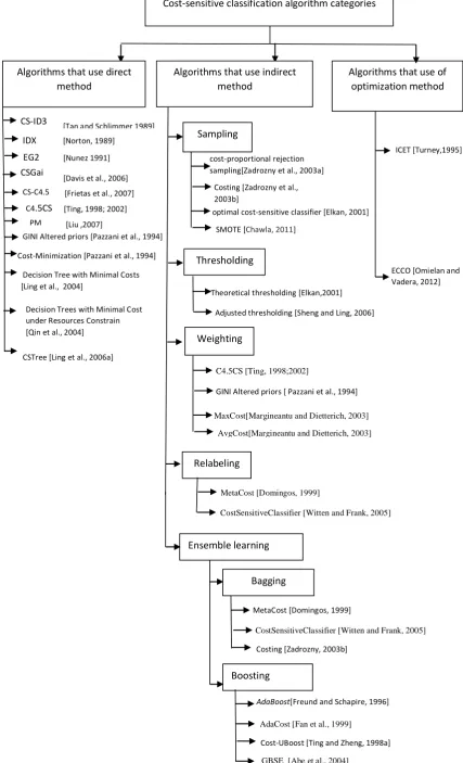
3.2.1 Cost sensitive algorithms categories ... 41

3.2.1.1 Algorithms that use direct methods ... 44

3.2.1.2 Algorithms that use indirect methods ... 46

3.2.1.2.1 Sampling ... 46

3.2.1.2.2 Thresholding ... 52

3.2.1.2.3 Weighting ... 53

3.2.1.2.4 Relabeling ... 54

3.2.1.2.5 Ensemble learning methods ... 55

3.2.1.3 Algorithms that use optimization methods ... 58

3.3 Literature review of research on cost-sensitive Bayesian network algorithms ... 59

3.4 Summary ... 62

Chapter 4: Cost-Sensitive Bayesian Network Learning Algorithms ... 63

4.1 Learning cost-sensitive Bayesian networks via a sampling approach ... 63

4.2 Learning cost-sensitive Bayesian networks via an amending approach ... 66

4.2.1 Amending the formula for learning the structure ... 68

4.2.2 Amending the formula for learning parameters... 68

4.3 Learning cost-sensitive Bayesian networks via Genetic algorithms ... 71

4.3.1 Encoding tree augmented networks ... 71

4.3.2 Fitness Function ... 73

4.3.3 Evolving the populations ... 74

4.4 Summary ... 79

Chapter 5: An Empirical Evaluation of the New Algorithms for Learning Cost-Sensitive Bayesian Networks ... 80

5.1 Empirical comparison results ... 80

5.1.1 Datasets ... 81

5.1.2 Experiment methodology ... 83

5.1.3 Experiments ... 85

5.1.3.1 Experiment 1: CS-BN using the sampling approach ... 88

5.1.3.2 Experiment 2: CS-BN using the amending approach ... 92

iii

5.3 Summary ... 96

Chapter 6: Conclusions and Future Work ... 97

6.1 The research objectives revisited ... 98

6.2 Limitations and future work ... 101

References ... 103

Appendix A ... 114

A1: Connections in a BN structure ... 114

A2: Example to illustrate Propagation of information in the Alarm problem... 115

Appendix B ... 119

B1: Example of learning a TAN using the play-tennis dataset ... 119

B2: Example of using a TAN as a classifier for the play-tennis dataset ... 126

Appendix C ... 127

C1: Summary of Implementation and Class Diagrams... 127

iv

Figure 1.1: Propagation and the impact of evidences (Pearl, 1988; 2014). ... 2

Figure 1.2: How cost-insensitive classification algorithms work (Fan et al., 2002). ... 4

Figure 1.3: Research methodology. ... 9

Figure 2.1: Classification process (Han et al., 2015). ... 12

Figure 2.2: A simple Bayesian network for fraud detection (Ezawa and Schuermann, 2015) ... 14

Figure 2.3: Illustration of three dependency events (Sawaal, 2015). ... 16

Figure 2.4: Illustration of two independency events (Sawaal, 2015). ... 16

Figure 2.5: Conditional probability example (Kountz et al., 2011). ... 17

Figure 2.6: BNs’ structure of lung cancer problem using Netica. ... 20

Figure 2.7: Types of inferences ... 21

Figure 2.8: Bayesian network structures. ... 23

Figure 2.9: Bayesian network structure learning approaches. ... 24

Figure 2.10: Set of operators (Vandel et al., 2012). ... 26

Figure 2.11: Model selection that maximize the score given data (Meek, 2015)... 27

Figure 2.12: Illustration of the concept of data compression in MDL (Rish, 2015). ... 30

Figure 2.13: How MWST finds a tree with the greatest total weight (Hong, 2007). ... 33

Figure 2.14: A simple BNs model with CPTs. ... 36

Figure 2.15: A simple network structure for the play-tennis dataset and the associated CPTs... 37

Figure 3.1: Cost-sensitive learning categories ... 43

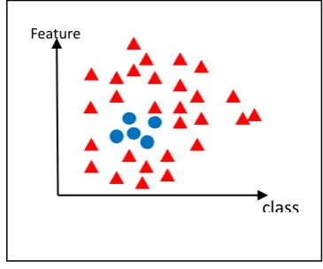
Figure 3.2: Imbalanced dataset ... 47

Figure 3.3: Sampling with / without replacement (WIKIbooks, 2015) ... 49

Figure 3.4: Costing algorithm based on Cost-proportionate rejection sampling with aggregation. ... 51

Figure 3.5: The best threshold is the point that gives minimum cost (Sheng and Ling, 2006). ... 53

Figure 3.6: The MetaCost system (Domingos, 1999)... 56

Figure 3.7: Illustration of boosting method (UCSD, 2015). ... 57

Figure 3.8: Cost-sensitive boosting (composite hypothesis ) (UCSD, 2015). ... 58

Figure 3.9: The ICET System (Turney1995). ... 59

Figure 4. 1: Illustration of sampling approach steps with hepatitis dataset. ... 64

Figure 4.2: CS-BN algorithm using sampling. ... 65

Figure 4.3: An illustration of the altered probability. ... 67

Figure 4.4: CS-BN algorithm using the amending approach. ... 69

Figure 4.5: An illustration of how TAN classifier represents the genes. ... 71

v

Figure 4. 9: Nine steps to illustrate the main idea of CS-BN via GAs. ... 78

Figure 5.1: Discretising data (Fayyed and lrani, 1993). ... 81

Figure 5.2: The experiment methodology ... 84

Figure 5.3: Expected cost of CS-BN algorithms and existing algorithms ... 87

Figure 5.4: Accuracy of CS-BN algorithms and existing algorithms ... 88

Figure 5.5: Misclassification error if experiment 1 for breast cancer dataset ... 89

Figure 5.6: WEKA a pre-process stage shows the similarity and diversity of attribute variables ... 90

Figure 5.7: Misclassification error if experiment 2 for breast cancer dataset ... 92

Figure 5.8: CS-BN via GA reduces the number of misclassification error for the Breast Cancer dataset. ... 94

vi

Table 2. 1: Joint probability example. ... 18

Table 2.2: Number of BN structures based on number of nodes (Laskey, 2015). ... 25

Table 2.3: A simple play-tennis dataset with two attributes. ... 36

Table 3.1: A cost matrix for two-class problems ... 40

Table 3.2: Outcomes from decision tree classifier (J48) on the Breast cancer dataset. ... 41

Table 3.3: Summary of the literature review of cost-sensitive Bayesian network algorithms. ... 62

Table 5.1: The main characteristics of datasets used in the comparisons ... 82

Table 5.2: Cost matrix of two class labels C1=4, C2=1 ... 83

Table 5.3: Comparison between CS-BN algorithms and existing algorithms ... 86

vii

AI Artificial Intelligence

BD Bayesian Dirichlet

BDe Bayesian Dirichlet likelihood-equivalence

BDeu Bayesian Dirichlet likelihood-equivalence uniform joint distribution

BNs Bayesian Networks

CI Conditional Probability Tables

CL tree Chow-Liu tree

CLL Conditional log likelihood CSC

CS-BN

CostSensitiveClassifier

Cost-sensitive Bayesian networks

DT Decision tree

ECCO Evolutionary Classifier with Cost Optimization

FN False Negative

FP False Positive

GAs Genetic Algorithms

ICET Inexpensive Classification with Expensive Test

LL Log-Likelihood

MC+BN MetaCost classifier used Bayesian network algorithm TAN as base classifier MC+J48 MetaCost classifier used decision tree algorithm J48 as base classifier.

MDL Minimum Description Length

MI Mutual Information

MWST Maximum Weight Spanning Tree

SE Simple Estimator

TANs Tree Augmented Naïve-Bayes networks

TN True Negative

TP True Positive

UML Unified Modelling Language

 Bayesian parameters

G Graph

P(j|x) The probability estimation of classifying the instance x into class j

Cost(i, j) The cost of misclassification of class i

ICFA Information Cost Function for an attribute A

viii

First of all, I would like to thank ”ALLAH ALMIGHTY” who has given me the strength, patience and knowledge to continue and finish my PhD journey which started as an idea and led to a four-year-long study process. It would not have been possible to write this PhD thesis without the help and support of the kind people around me, to only some of whom it is possible to divulge particular mention here. I would like to express my deepest sense of gratitude to my great supervisor Professor Sunil Vadera for his assistance, support and feedback during this research, as well as his help in pointing me in the right direction. After four years of patience and hard work, my dream has really come true following his support. Therefore, I need to state that the congratulation compliments which I may receive should be extended to him.

Special thanks to my fabulous family, especially my parents, sisters, and brothers who have pushed themselves to the extreme ends to ensure that I continue my education to the highest level. I have a special feeling of gratitude towards my husband, who formed my vision and encouraged me in achieving my goal, through continued patience at all times. I wish to record my special thanks and gratitude to my wonderful daughters Ranim and Ratil and to my delightful son Mohammed, for being there for me throughout the entire doctorate programme. Truly, without their love and support, I would not have reached this point in my life and this PhD research work would not have been possible.

I would like to extend a huge, warm thanks to my friends, Dr. Haya Alshehri, Dr. Rabea Elmazuzi, and Dr. Majda Elferjani; they were always by my side during difficult situations and they have always supported and encouraged me.

ix

External Publications

Nashnush, E. and Vadera, S. (2014). Cost-Sensitive Bayesian Network Learning Using Sampling. In Recent Advances on Soft Computing and Data Mining. Springer International Publishing, pp. 467-476.

Nashnush, E. (2014). Cost-Sensitive Bayesian Network algorithms . Libya Higher Education Forum. “A Vision for the Future”.http://libyaed.com/ .5 - 6 June 2014, London.

Nashnush, E. and Vadera, S. (2014). Learning Cost-Sensitive Bayesian Networks via Direct and Indirect Methods. Integrated Computer-Aided Engineering Journal, (in process, it has been submitted on 30 September 2014).

Nashnush, E. and Vadera, S. (2015). EBNO: An Algorithm for Evolving Cost-Sensitive Bayesian Networks. ACM journal on Knowledge Discovery from Data (TKDD), (in process, it has been submitted on 28 April 2015).

Internal Publications

Nashnush, E. and Vadera, S. (2012). Cost-Sensitive / Insensitive Learning algorithms. 3rd Computing Science and Engineering Post Graduate Conference, Salford University, UK. Nashnush, E. and Vadera, S. (2013). Direct and indirect approaches for learning cost-sensitive Bayesian network. 4th Computing Science and Engineering Post Graduate Conference, Salford University, UK.

*_{Nashnush, E. and Vadera, S. (2013). Cost-Sensitive Bayesian Network Learning Algorithm.}

Salford Postgraduate Annual Research Conference 2013 (SPARC 2013), 5-6 Jun 2013, University of Salford, UK.

Nashnush, E. and Vadera, S. (2013). Cost-Sensitive Bayesian Network learning using Sampling approach. Dean’s Annual Research Showcase, Poster and abstract. Salford University, UK.

Nashnush, E. and Vadera, S. (2015). Three approaches for Cost-sensitive Bayesian Network algorithm. A Three Minute Thesis at the 2015 Salford Postgraduate Annual Research Conference (SPARC 2015), Salford University, UK.

Nashnush, E. and Vadera, S. (2015). Using Genetic Algorithms to optimize Tree Augmented Naïve Bayes classifier. Dean’s Annual Research Showcase. Poster and abstract. University of Salford, UK.

x

Bayesian networks are becoming an increasingly important area for research and have been proposed for real world applications such as medical diagnoses, image recognition, and fraud detection. In all of these applications, accuracy is not sufficient alone, as there are costs involved when errors occur. Hence, this thesis develops new algorithms, referred to as cost-sensitive Bayesian network algorithms that aim to minimise the expected costs due to misclassifications. The study presents a review of existing research on cost-sensitive learning and identifies three common methods for developing cost-sensitive algorithms for decision tree learning. These methods are then utilised to develop three different algorithms for learning cost-sensitive Bayesian networks: (i) an indirect method, where costs are included by changing the data distribution without changing a cost-insensitive algorithm; (ii) a direct method in which an existing cost-insensitive algorithm is altered to take account of cost; and (iii) by using Genetic algorithms to evolve cost-sensitive Bayesian networks.

1

Chapter 1: Introduction

This chapter presents the thesis introduction and methodology. Section 1.1 provides an introduction of classification algorithms and Bayesian network algorithms. Section 1.2 presents the problem definition and the motivation for study. Section 1.3 presents the research questions, while Section 1.4 describes the research methodology that used. Section 1.5 explains the research hypothesis, aims and objectives and finally, Section 1.6 outlines the structure of the thesis.

1.1 Introduction

Classification is one of the most important methods in data mining, which plays an essential role in data analysis and pattern recognition, and requires the construction of a classifier. A classifier can predict the class label for an unseen instance from a set of attributes. As Friedman (1997) states:

“The induction of classifiers from datasets of pre-classified instances is a central problem in machine learning”.

2

An important feature of Bayesian networks is the way it propagates the impact of new evidence, providing each node with a belief vector that is consistent with the axioms of probability theory (Pearl, 1988; 2014). For example, the diagram in Figure 1.1 shows a simple example, presented by Pearl (2014), to model an alarm problem with a Bayesian network: if somebody calls you and informs you that your alarm has gone off, you might think there is a burglar in your home, and you will go to your home directly. On your way, if you hear a radio announcement that there was an earthquake nearby, you might reconsider given that the earthquake may have caused the alarm. In particular, from this information, the BNs can propagate the impact of evidence from effect to cause (Radio Earthquake), then from cause to effect (Earthquake  Alarm), and then again from effect to cause (Alarm  Burglary). In this figure, A represents Alarm and B represents Burglary, the impact of the evidence from the Radio announcement will be to update the beliefs so that AB less credible.

Figure 1.1: Propagation and the impact of evidences (Pearl, 1988; 2014).

Over the last few years, Bayesian networks have become very popular. Bayesian networks and their algorithms are explained by Pearl (2001), who won the Association for Computing Machinery Turing Award in 2012. Moreover, Bayesian networks have been successfully applied in different areas to create consistent probabilistic representations of uncertain knowledge in several fields, including: medical diagnosis (Spiegelhalter et al., 1989; Heckerman et al., 1995), image recognition (Booker and Hota, 2013), language understanding (Charniak and Goldman,1989), search algorithms (Hansson and Mayer, 1989). In particular, the book by Pourret et al. (2008) and Kenett (2012) describes 21 applications of Bayesian networks to illustrate their wide range of applications in clinical decision support,

A

Alarm Burglary

Radio

announcement Earthquake

3

complex genetic models, crime risk factor analysis, inference problems in forensic science, terrorism risk management, credit rating of companies, and enhancing human recognition.

In machine learning algorithms, several studies have mentioned that, learning processes should take account of the costs involved in decision-making (Breiman et al., 1984; Turney,1995, 2000; Zadrozny, and Elkan, 2001). Turney (2000) lists the kind of costs that should be considered, such as cost of misclassification, the cost of test, the computational cost, data acquisition cost, active learning cost, human computer interaction cost, and cost of teacher. Amongst these, the misclassification cost is one of the most important. In fact, misclassification cost happens when, the examples that belong to negative class are classified to positive class (FP; classifying a negative example as positive), or the examples that belong to positive class are classified to negative class (FN; classifying a positive example as negative). For example, in a credit card fraud detection application, if the system classifies a transaction of a customer as a non-fraud when fraud has occurred, it is likely to result in financial loss. In contrast, if a system classifies a transaction as a fraud when it is not the costs would involve some further checks before proceeding with the transaction.

This observation has led to many recent studies focusing on cost-sensitive learning algorithms. Historically, most of the cost-sensitive algorithms developed have focussed on learning decision trees, with a recent survey comparing over 50 algorithms (Lomax and Vadera, 2013). In contrast, little attention has been paid to developing cost-sensitive Bayesian networks (Gao, et al., 2008; Nashnush and Vadera 2014; Jiang and Wang, 2014; Kong et al. 2014). Hence, the main focus of this thesis is to study whether it is possible to develop a new machine learning algorithm to learn Bayesian Networks that can perform cost-sensitive classifications.

1.2 Motivation

4

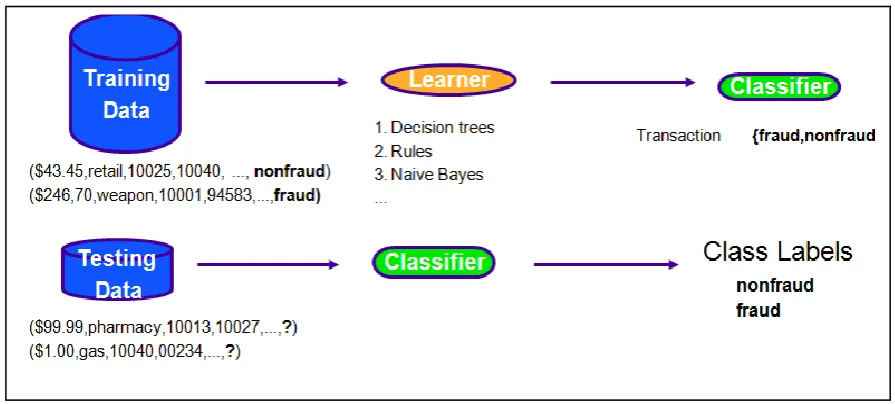
particular, in traditional machine learning classification algorithms such as decision tree induction, neural networks, Bayesian networks, the aim is to build a model using a training set, and then use the model for classifying unseen cases. Figure 1.2 shows such an example, where some training data is used as input to a learning algorithm, which classifies whether there has been a fraudulent transaction. Historically, most of these techniques only focus on predicting correct results and maximising accuracy. More recently, as mentioned above, there has been recognition that costs play an important role and should be taken into account when developing classification algorithms. In particular, in real world applications, one should take into consideration misclassification costs (Turney,2000).

Figure 1.2: How cost-insensitive classification algorithms work (Fan et al., 2002).

Cost-sensitive learning is a type of learning in data mining that takes account of costs such as misclassification costs, test costs, or any other costs into consideration (Turney, 2000), and aims to minimize total costs by treating the different classification errors differently (Ling et al., 2006). On the other hand, cost-insensitive learning, does not take the misclassification costs into consideration and focuses on accuracy only.

5

increase the accuracy will be biased to classify instances to most frequent case (He and Garcia, 2009). The following examples illustrate the need to take account of costs:

 To detect a fraudulent customer, the cost of misclassifying a customer who commits fraud (rare class) is greater than the cost of misclassifying a customer who is non-fraudulent (common class).

 Also, in a medical application, the cost of misclassifying a patient who has cancer is greater than the cost of misclassifying a patient who does not have cancer.

In these types of domain, building a classifier that does not consider the cost of misclassification is unlikely to perform well because it will be biased towards the instances under the category of the frequent class, which will result in producing a useless classifier. Thus, cost-sensitive learning algorithms that take costs into consideration and deal with different types of cost differently are essential (Charles and Victor, 2008).

Hence, a number of authors, who recognised the need for taking account of costs, have focussed on developing cost-sensitive decision tree learning algorithms, including : Cost-Minimization (Pazzani et al., 1994), Decision Tree with Minimal Costs (Ling et al., 2004), EG2 (Núñez, 1991), CS-ID3 (Tan and Schlimmer, 1989), IDX (Norton 1989), CS-C4.5 (Frietas et al., 2007), CSNL (Vadera, 2010). All of these algorithms use the cost directly during the algorithm process. In contrast, some of the algorithms use the cost indirectly, before and after using the algorithm, such as Costing (Zadrozny et al., 2003b), C4.5CS (Ting, 2002), MaxCost (Margineantu and Dietterich, 2003), MetaCost (Domingos, 1999), CostSensitiveClassifier (CSC) (Witten and Frank, 2005),and AdaCost (Fan et al., 1999).

Although Bayesian networks have been successfully applied, there has been little, but no research on optimising them for cost-sensitive learning. Hence, this thesis explores the potential for learning Bayesian networks for cost-sensitive classification.

1.3 Research aims and objectives

6

algorithms, including existing sensitive decision learning tree algorithms, existing cost-sensitive Bayesian network learning algorithms, and existing cost-incost-sensitive Bayesian network learning algorithms.

To check this hypothesis, this research aims to develop methods that learn Bayesian networks that take account of misclassification costs and then utilise empirical methods to assess the extent to which the hypothesis is true. The specific research objectives are:

1. To review the background of Bayesian networks learning algorithms, and analyse the types of this algorithm.

2. To review the literature on cost-sensitive learning, analyse the most significant issues in current cost-sensitive learning algorithms, and identify the strategies used.

3. To develop new cost-sensitive Bayesian network learning algorithms that aim to overcome the issues identified, and are based on methods of cost-sensitive learning algorithms such as direct, indirect, and optimization methods.

4. To evaluate the new algorithms against existing cost-sensitive algorithms and measure performance, and compare the algorithms in terms of accuracy, and cost minimization.

1.4 Research questions

Given the above aims and objectives, the following key questions need to be addressed when attempting to design algorithms to learn Bayesian networks that take account of costs. In relation to the research aims and objectives, each question is answered in Section 1.3:

Q1. How can a learning Bayesian algorithm involve misclassification costs?

This question is answered in objectives 1, 2 and 3 by analysing Bayesian networks algorithm, and based on the methods that used to involve costs into decision trees algorithms. Hence, the new Bayesian networks algorithms can involve misclassification costs in three different methods; direct, indirect, and optimization method.

Q2. At which stage should Bayesian networks include these costs: before construction, during construction, during learning parameters or after final construction?

7

Bayesian networks algorithm (learning structure, and learning parameters), and based on the ways that used in cost-sensitive decision trees algorithms. Hence, new Bayesian networks algorithms can include misclassification cost before construction by using sampling approach; or during learning structure and parameters by using amending approach.

Q3. How can the costs be balanced against the need to maintain the accuracy rate?

This question is answered in objectives 3, and 4 by including the costs in the right place without changing the performance of the algorithms then evaluate these algorithms against existing cost-insensitive and sensitive algorithms.

Q4. What are the weaknesses of existing cost-sensitive Bayesian algorithms?

This question is addressed in objectives 2 by analysing the most significant issues in current cost-sensitive Bayesian networks algorithms.

1.5 Research methodology

This section describes the research methodology that used in this research, and shows the outline of the methodology adopted in this thesis. As Rajasekar et al. (2006) describe, there is a difference between research methods, and research methodology. Essentially, research methods represent all the methods, procedures, and schemas, which are used by a researcher during a research study. For example, these methods might be collecting and sampling data, using some hypotheses, and finding a solution to a problem. Also, any research that is based on experiments requires collection of facts, measurements, hypotheses, and observations, and these are called scientific research methods. Given the nature of this thesis, which is focussed on objective quantitative measures (Rajasekar et al., 2006; Kothari, 2011), this PhD research uses the quantitative research methodology because it is based on testing new hypotheses.

8

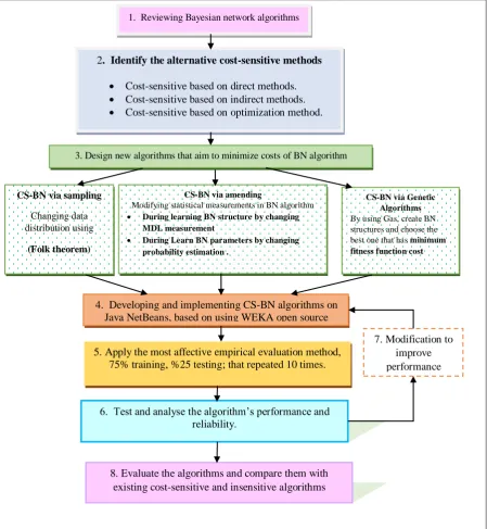
1. Starting with reviewing the background of Bayesian networks. The objective 1 can be achieved in this phase.

2. Identify the alternative cost-sensitive methods by studying the literature review of existing cost-sensitive algorithms that based on three methods; indirect; direct, and optimization method. Where, the objective 2 can be achieved in this phase.

3. Design new algorithms that aim to minimize misclassification costs, these algorithms are based on three methods that show in phase 2.

4. Implement CS-BN algorithms, where, this study used the open source algorithms in the data mining system WEKA, which were developed by Hall et al. (2009). The algorithms are implemented in java NetBeans.

5. The empirical evaluation methodology adopted to split the datasets into 75% for training and 25% for testing, and to apply the algorithms10 times randomly with 16 misclassification costs from 1 to 4 for each class label. Then, the average performance of each algorithm with standard errors are calculated 10 times (Gurland and Tripathi, 1971).

6. Test and analyse the algorithm’s performance and reliability; to test the algorithms, benchmark datasets from UCI repository datasets (Asuncion and Newman, 2007) have been used to simulate problems of cost-insensitive algorithms.

7. The algorithms are modified to improve the performance. These algorithms are modified throughout the study, feedback from the supervisor, examiners, assessments, conferences, and journals have been taken into account. Hence, the objectives 3 can be achieved in phases 3 ,4, 5,6, and 7.

9

Figure 1.3: Research methodology.

1.6 Thesis organisation

The thesis is organised into six chapters, set out as follows: Chapter 1: Thesis introduction and methodology

This chapter presents a brief introduction to the research, introducing the reader to the problem statement and motivation, potential contribution, research methodology, research hypothesis, aims and objectives.

8. Evaluate the algorithms and compare them with existing cost-sensitive and insensitive algorithms

CS-BN via sampling

Changing data distribution using

(Folk theorem)

CS-BN via amending

Modifying statistical measurements in BN algorithm

 During learning BN structure by changing

MDL measurement

 During Learn BN parameters by changing

probability estimation .

CS-BN via Genetic Algorithms

By using Gas, create BN structures and choose the best one that has minimum fitness function cost

1. Reviewing Bayesian network algorithms

2. Identify the alternative cost-sensitive methods  Cost-sensitive based on direct methods.

 Cost-sensitive based on indirect methods.

 Cost-sensitive based on optimization method.

4. Developing and implementing CS-BN algorithms on Java NetBeans, based on using WEKA open source

6. Test and analyse the algorithm’s performance and reliability.

7. Modification to improve performance

3. Design new algorithms that aim to minimize costs of BN algorithm

10

Chapter 2: Background on Bayesian networks

This chapter presents the basic of data classification process, the background to Bayesian network learning algorithms and basic laws of probabilities. It shows types of Bayesian network algorithms with examples, how they learn a BNs structure, and how they learn the parameters.

Chapter 3: Survey of existing cost-sensitive algorithms

This chapter includes a survey of existing cost-sensitive learning algorithms; it shows the categories of cost-sensitive learning algorithms, direct, indirect, and optimization algorithms, and literature review in cost-sensitive Bayesian network algorithms.

Chapter 4: The development of cost-sensitive Bayesian network learning

This chapter presents the development of three new algorithms for learning cost-sensitive Bayesian networks; these algorithms based on, (i) indirect methods by changing the data distribution to reflect the costs, (ii) direct methods by amending an existing algorithm, (iii) optimization method by using Genetic algorithms to create a BN structures that has minimum fitness function cost.

Chapter 5: An empirical evaluation of the new algorithms for learning cost-sensitive Bayesian networks

This chapter presents a comprehensive empirical evaluation, including a comparison with existing cost-sensitive/ insensitive learning algorithms, and finally, evaluating and analysing their performance by using the average cost and accuracy rates as measurements.

Chapter 6: Conclusions and future works

This chapter summarises the aims of this work and concludes with the achievements, including reflections on the extent to which the research objectives have been met and future developments that may be necessary.

Bibliography: It presents all the references in this thesis.

11

Chapter 2: Background on Bayesian Networks

This chapter presents an overview of Bayesian networks and the basic laws of probabilities. Section 2.1 describes the basics of the data classification process. Section 2.2 presents an overview of Bayesian networks, while Section 2.3 presents the principles of Bayesian networks such as probability, and inference. Section 2.4 presents algorithms for learning Bayesian networks. Finally, a summary of the chapter is presented in Section 2.5.

2.1 Data Classification

Data mining is an active research area involving the development and analysis of algorithms for extracting interesting knowledge and patterns from real-world datasets and summarizing it into useful information (Witten and Frank, 2005). Classification is one of the most important methods in data mining which plays an important role in data analysis, pattern recognition, and decision making (Aggarwal, 2014).

Classification requires the construction of a model that can be used to predict a class label for an unseen instance from a set of attributes. Classification algorithms attempt to learn the relationship between a set of variables (features) and a class label (target variable). In

particular, classification algorithms learn from training instances to construct a model; where

each instance is associated with a known class label. Then, in a testing phase, the model can

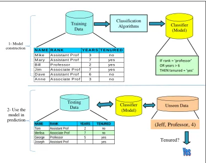
be used to assign labels to unlabelled test instances (Aggarwal, 2014). Figure 2.1 shows how

the classification process can be divided into two steps:

i. Model construction: training data is used to create a model, where the model is

represented in some forms such as classification rules, decision trees, Bayesian

networks, or mathematical formulae.

ii. Model usage: the model is used for classifying unseen or unknown instances, and

12

Figure 2.1: Classification process (Han et al., 2015).

Classification algorithms have been used in several applications, such as: customer target marketing (Rygielski et al., 2002), medical disease diagnosis (Cios and Moore, 2002), supervised event detection (Zhang et al., 2010), multimedia data analysis (Kantardzic, 2011), biological data analysis (Bishop, 2006), and social network analysis (Aggarwal, 2014). There are several techniques used for data classification such as:

 Decision trees algorithms that use a decision tree that is learned from labelled training instances (Quinlan, 1986).

 Rule-based algorithms for classifying examples using a collection of ”if -then” rules (Cohen,1995).

 Instance based algorithms that perform classification using only specific instances

(Aha et al., 1991).

 Neural networks algorithms that use a computational model based on biological neural networks (Funahashi, 1989).

NAME RANK YEARS TENURED

Tom Assistant Prof 2 no

Merlisa Associate Prof 7 no

George Professor 5 yes

Joseph Assistant Prof 7 yes

Testing Data Classifier

(Model)

Unseen Data

(Jeff, Professor, 4)

Tenured?

2- Use the model in prediction

1- Model construction

Classification Algorithms

IF rank = ‘professor’ OR years > 6 THEN tenured = ‘yes’

Classifier (Model) Training

Data

N A M E R A N K Y E A R S T E N U R E D

M ik e A ssistan t P ro f 3 n o

M ary A ssistan t P ro f 7 yes

B ill P ro fesso r 2 yes

J im A sso c iate P ro f 7 yes

D ave A ssistan t P ro f 6 n o

A n n e A sso c iate P ro f 3 n o

13

 Bayesian networks algorithms that are statistical classifiers and are based on Bayes theorem (Pearl, 1988; 2014).

This thesis focuses on Bayesian networks, and hence the following sections describe the foundation for Bayesian networks. Section 2.2 provides an introduction to the main concept, Section 2.3 describes the main principles of probabilities used when performing classification, and Section 2.4 describes algorithms that learn Bayesian networks.

2.2 Overview of Bayesian networks

Bayesian networks, which were invented in 1988 by Judea Pearl, changed the focus of AI from logic to probability. In the last decade, Bayesian networks have become one of the most popular tools to structure uncertain knowledge. Indeed, Bayesian networks have been successfully used in a number of fields including medical diagnostic systems (Spiegelhalter et al., 1989; Heckerman et al., 1995), in NASA AutoClass project for data analysis and control the space shuttle (Morris, 2003), Fraud detection systems(Maes et al., 2002), and Speech recognition systems (Zweig and Russell, 1998).

14

(in)dependence between nodes that will be described later in Section 2.3.1). Where a direct edge represents the direct influence between nodes (statistical dependency), while an indirect edge of nodes that are not connected, represents the indirect influence between nodes (statistical conditional independency) (Corani et al., 2012), where direct and indirect influence will be described later in Section 2.3.2.2.

More specifically, in BNs’ structures each node has a set of values, and the relationship between the node and its parents is defined by a conditional probability table (CPT). This table determines the probabilities of the values between a stated node given its parents. For example, Figure 2.2 shows a simple fraud detection Bayesian network, with CPTs of fraudulent transactions which are more likely to happen when the card holder is travelling abroad because tourists are targets for thieves, as travel and fraud are causes for foreign purchase. Invariably, travel explains foreign purchase, thus is evidence against fraud, while the network has three nodes, representing Travel, Fraud, and Foreign purchase, respectively. The travel node, as being a parent node has a prior probability table that indicates the chances of someone travelling to be 0.05 and not travelling to be 0.95. Additionally, the table for the Fraud node shows the probability of fraud given values of its parent node, Travel. Thus, the probability of fraud for someone travelling is 0.01, and 0.002 if it is not travelling. While, the probability of no fraud for someone travelling is 0.99, and 0.998 if not travelling. This is very similar to the Foreign Purchase node.

Figure 2.2: A simple Bayesian network for fraud detection (Ezawa and Schuermann, 2015)

Given such a network, it can be used to update when evidence is made available. For example, if one knows that a person is travelling (Travel is True), the probabilities of Fraud

Travel True False

True 0.01 0.99

False 0.002 0.998 Fraud

Foreign purchase

True False

0.05 0.95 Travel

Travel Fraud True False

True True 0.90 0.10

False True 0.10 0.90

True False 0.90 0.10

15

given Travel to be true and false become 0.01 and 0.99 respectively. Also, the Foreign Purchase node is updated to 0.90, and 0.10 when the Foreign Purchase are true and false respectively.

2.3 Principles of Bayesian networks

This section describes the key principles of Bayesian networks, while, Section 2.3.1 summarises some definitions from probability theory including Bayes rule which is central to Bayesian networks, and also presents the notions of dependence and independence. Section 2.3.2 explains the basic of BNs, also how the information is propagated in BNs, and shows how to use statistical inference based on the Bayes rule to update the probability for a hypothesis as evidence is acquired.

2.3.1 Definitions from probability theory

This section describes the basic laws of probabilities and shows how to calculate the probability distribution between two events based on whether they are dependent or independent events. A probability function P(A) of an event A, represents the density function of A, while, a joint probability P(A,B) is the probability of two events, A and B, occurring together at the same time.

2.3.1.1 Dependency events

Formally, if two events are dependent, namely they do influence each other in any way, then:

𝑃(𝐴, 𝐵) = 𝑃(A ∩ B) = P(A) ∗ P(B after A) (2.1) where A, and B are dependent

In particular, if the two events are considered dependent, then the outcome of the one event depends on the probability of the other event )Ben‐Gal, 2007). For example, if one has a bag that contains 4 balls green, 2 balls red, and 1 ball blue, where in each time we have to choose one ball without replacement, then each event is dependent on the other events as illustrated in Figure 2.3, and according to equation (2.1) the probability of choosing green and red is:

P(Green, Red) = P(Green) ∗ P(Red after Green) = 4

7 ∗ 2

6=

8

16

Figure 2.3: Illustration of three dependency events (Sawaal, 2015).

2.3.1.2 Independency events

Formally, if two events are independent, namely they do not influence each other in any way, then:

𝑃(𝐴, 𝐵) = P(A) ∗ P(B) (2.2) where A, and B are independent

If the two events are considered independent, then subsequently each can occur individually and the outcome of one event does not rely on the other. Hence, this will occur if the fact A occurring does not affect the probability of B occurring (Ben‐Gal, 2007). For example, this can be noted if one has 2 events; choosing a random card from 5 cards, and rotating a wheel has 8 parts, where both of events are independent. According to equation (2.2), the probability of choosing card number 10 and rotating a wheel on part 6 is:

P(Card 10, Wheel on 6) = 1

5∗ 1

8=

1

40 = 0.025

Figure 2.4: Illustration of two independency events (Sawaal, 2015).

P(green)= 4/7 P(Red)= 2/7 P(blue)= 1/7

P(green)= 3/6 P(Red)= 2/6 P(blue)= 1/6 After choosing green

without replacement

17

2.3.1.3 Conditional probability

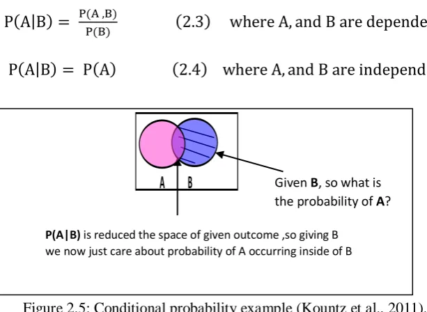
If two events are dependent, then we have to use the concept of conditional probability. Conditional probability is the probability of an event (A) occurring, given that another event (B) has already occurred. The conditional probability reduces the sample space of giving the outcome. Formally, conditional probability can be defined by:

P(A|B) = P(A ,B)

P(B) (2.3) where A, and B are dependent.

P(A|B) = P(A) (2.4) where A, and B are independent.

Figure 2.5: Conditional probability example (Kountz et al., 2011).

Bayes’s theorem was introduced by Thomas Bayes (1701 - 1761) and represents how the conditional probability of a set of possible causes for given an observed outcome. In particular, this theorem is used for statistical inference (Bolstad, 2013), and it is stated mathematically as:

𝑃(𝐴|𝐵) = 𝑃(B|A)𝑃(A)

𝑃(𝐵) (2.5)

Where:

 A and B are events, and B is observed.

 P(A) is prior probability

 P(B) is observed probability.

 P(B|A) is a likelihood probability; the conditional probability of B given that A is true.

 P(A|B) is a posterior probability; the conditional probability of A given that B is true, it reflects the belief about the hypothesis after B has been observed.

For example, to calculate the probability of someone who has brown hair and given female, when given the Table 2.1:

Given B, so what is the probability of A?

P(A|B) is reduced the space of given outcome ,so giving B we now just care about probability of A occurring inside of B

18

Total = 11 Female Male Brown hair 3 4

Blond hair 2 2

Table 2. 1: Joint probability example.

P(Brown hair |Female) = P(Brown hair ∩ Female)

P(Female) =

3 11 ⁄ 5

11

⁄ =

3

5= 0.6

2.3.2 Bayesian networks structure

This section presents the concept of Bayesian networks; where Section 2.3.2.1 shows how to use BNs model joint distributions of a set of variables, and how BNs use conditional probabilities between nodes (variables) to compute the probability of events. It presents the Chain theorem which is used to calculate the joint probability distribution over sets of random variables in the BNs structure. Section 2.3.2.2 demonstrates how to use Bayes’s theorem to enable inference when certain pieces of evidence are available to answer queries and update beliefs.

2.3.2.1 Bayesian networks basics

19

Formally, a Bayesian network is represented as DAG that encodes a joint probability distribution over a set of random variables X. This shows as a pair of graph G and parameters

 B=<G, >, where G is a DAG of n random variables 𝑋 = {𝑥1, 𝑥2 , 𝑥3, … . , 𝑥𝑛}, and the

graph G encodes independence assumptions; each variable 𝑥_𝑖 is independent of its non-descendants given its parents in G. While,  represents the set of parameters between the nodes. In particular, a parameter of each node 𝑥_𝑖 in 𝑋, is represented as 𝑃(𝑥_𝑖|_𝑥𝑖), where_𝑥𝑖 is the set of parents of node 𝑥𝑖. More precisely, a BN uses a chain theorem to calculate the

joint probability distribution over sets of random variables, as demonstrated in equation (2.6). It is best to let a BN be a Bayesian network over variables, 𝑋 = {𝑥1, 𝑥2 , 𝑥3, … . , 𝑥𝑛}, as the

BN specifies a unique joint probability distribution P(X) given by the product of all conditional probability tables specified in the BN (Schum, 2001). Given that, by definition, each node 𝑥_𝑖 has a conditional probability distribution with its parent 𝑃(𝑥_𝑖|_𝑥𝑖), and the chain rule can be used to define the joint distribution as follows:

𝑃(𝑥1, 𝑥2 , 𝑥3, … , 𝑥𝑛) = ∏ 𝑃(𝑥𝑖|𝑥𝑖) 𝑖=𝑛

𝑖=1

(2.6)

For example, the network in Figure 2.2 (the Fraud example), can be used to model the joint distribution and to find what is the probability if someone is travelling, and will not receive a fraudulent transaction, and he will make foreign purchases. P( Travel=True, Fraud=False, Foreign Purchase=True) = P(Travel)*P(Fraud|Travel)*P(Foreign purchase| Travel,Fraud) = 0.05 * 0.99 * 0.90= 0.0445 .

More precisely, inference in a Bayesian network involves updating the probabilities of nodes’ given evidence and is described in the following section.

2.3.2.2 Bayesian inference

20

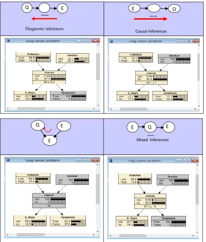
This network model is part of the lung cancer problem and can be used in scenarios, such as with a patient who visits a doctor with breathing difficulties (known as Dyspnoea) and is worried that he has lung cancer. A doctor also knows that other relevant information that increase the chances of cancer such as pollution, and smoking, as well as, a positive X-ray would indicate lung cancer. Consequently, through this scenario, there are four types of inference, as shown in Figure 2.7; where E is evidence node, and Q is query node:

Figure 2.6: BNs’ structure of lung cancer problem using Netica.

i. Diagnostic inferences (inference from effect to cause): This type of inference starts from effects to causes, and occurs in the opposite direction to the arcs, from effects to causes. For instance, in the above example, if one observes Dyspnoea, then, as illustrated in Figure 2.7(a), evidence propagates from symptoms Dyspnoea to Cancer, and then up to Pollution and Smoker, the results in propagation down from cancer to X-Rays (Korband and Nicholson, 2010). Comparatively, the process of going up from a child to its parents is illustrated in Figure 2.7(a).

ii.Causal inferences (inference from cause to effect): This type of inference starts from cause to effects as illustrated in Figure 2.7(b) where evidence is provided that a person smokes, then this is propagated down the arrows, from Smoker to Cancer, then to X_Rays and Dyspnea. The change in the probability of Cancer also results in propagation up to Pollution. Whereas, the process of going down from a parent to children, as illustrated in Figure 2.7(b), is known as causal inference.

21

going from a parent to parent through its children as illustrated in Figure 2.7(c), is known as intercausal inference.

iv. Mixed Inferences: This type of inference is mixed between different types of inferences, where any node might be a query or piece of evidence, thus this inference can combine the above types of inference, as shown in Figure 2.7(d).

Figure 2.7: Types of inferences

E Q

Causal Inferences

Evidenc e

……

Evidence

Q _E

Diagnostic inferences

……

( c): Intercausal Inferences

Q _E

E Mixed Inferences

E Q E

…..

( d): Mixed Inferences

22

2.4 Learning Bayesian networks

A Bayesian network can be used as a classifier by computing the posteriori probability of a set of labels given the observable features (Pearl, 1988), where to build a complete BN classifier, there are two aspects to constructing a BN (Neapolitan, 2004):

 learning the graphical structure (topology), which studies the qualitative part and how to find a graphical relationships between the variables.

 learning the parameters (conditional probability estimation), which studies how to quantify the relationships and how to determine the extent of the relationship between the variables and takes the form of a table that represents the conditional probabilit ies between a node and in its parents in CPT.

2.4.1 Bayesian network structure learning

23

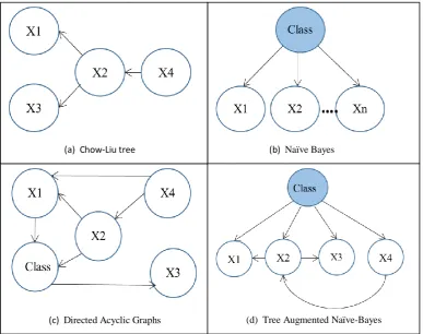
between attributes as shown in Figure 2.8(d). Given that a TAN improves upon Naïve Bayes by avoiding its conditional independence assumptions, avoids the computational overhead of a general Bayesian network, and has been shown to be an effective classifier (Friedman et al., 1997), thus, we adopt TANs in this study.

Figure 2.8: Bayesian network structures.

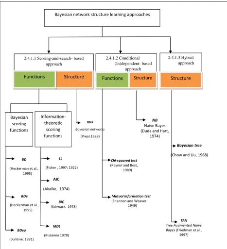
Historically, many Bayesian network structure learning algorithms have been developed, these algorithms generally fall into three approaches (Cheng and Greiner 1999):

 Scoring-and-search-based approach: find the BNs that maximizes score (Cooper and Herskovits,1992; Heckerman et al., 1995, Chickering, 2002).

 Constrain-based approach (CI-based approach): it called also Conditional Independent based algorithms, where it based on data by selecting for each variable a set of candidate parents (Spirtes et al., 1993; Cheng et al., 1997).

 Hybrid approach: that combines both of these approaches together to learn a BN structure.

(a) Chow-Liu tree

(c) Directed Acyclic Graphs (d) Tree Augmented Naïve-Bayes

24

Figure 2.9 presents a diagram that shows some references under each category and is followed by a description of the main categories (Carvalho, 2009; Cheng and Greiner, 1999).

Figure 2.9: Bayesian network structure learning approaches.

2.4.1.1 Scoring-and-search-based approach

The task of finding a structure of a Bayesian network that describes the observed data is difficult and time-consuming, and has been shown to be an NP-complete problem (Chickering1996, 2004). Practically, when the search space is extremely large, the search

NB

Naïve Bayes (Duda and Hart,

1974) Bayesian scoring functions Information-theoretic scoring functions BD (Heckerman et al.,

1995)

BDe (Heckerman et al.,

1995)

BDeu (Buntine, 1991)

LL (Fisher , 1997; 1922)

MDL (Rissanen 1978)

AIC

(Akaike, 1974)

BIC (Schwarz, 1978)

Chi-squared test (Rayner and Best,

1989)

Mutual Information test (Shannon and Weaver

1949)

Bayesian tree

(Chow and Liu, 1968)

TAN Tree Augmented Naïve Bayes (Friedman et al.,

1997)

BNs

Bayesian networks

(Preal,1988)

Bayesian network structure learning approaches

2.4.1.3 Hybrid approach Structure 2.4.1.2 Conditional (In)dependent- based approach

Functions Structure 2.4.1.1 Scoring-and-search- based

approach

25

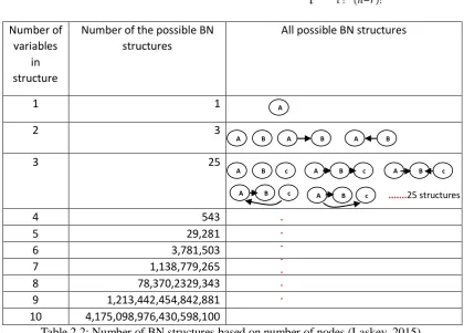
procedure will spend a lot of time examining unreasonable candidate structures, where the search space represents all the possible BNs structures. For example, Table 2.1 shows all possible structures of directed acyclic graphs (DAGs) given the number of variables (nodes) in the domain. Thus, when the number of nodes are large, then the number of possible DAGs are extremely large. Robinson (1973, 1977) derived the following efficiently computable recursive function to determine the number of possible structures that contain n nodes:

𝑓(𝑛) = ∑ (−1)𝑖+1_𝐶

𝑖𝑛2𝑖(𝑛−𝑖)𝑓(𝑛 − 𝑖) (2.7) 𝑛

𝑖=1

Where, n represents the number of variables, and 𝐶_𝑖𝑛 is (𝑛

𝑖)= 𝑛! 𝑖 ! (𝑛−𝑟)!

Number of variables

in structure

Number of the possible BN structures

All possible BN structures

1 1

2 3

3 25

4 543

5 29,281

6 3,781,503

7 1,138,779,265

8 78,370,2329,343

9 1,213,442,454,842,881 10 4,175,098,976,430,598,100

Table 2.2: Number of BN structures based on number of nodes (Laskey, 2015).

Cooper (1990) argued that given this is an NP-hard problem, we need to find "approximate solutions". The first attempts at finding approximate solutions were by Chow-Liu (1968) who developed branching algorithms to learn Bayesian trees. Dagum and Luby (1993) showed that even finding approximate solutions is NP-hard, thus they introduced a new method that restricted the possible parents of each node. After that, Dasgupta (1999) introduced 2-polytrees (a singly connected network) which is also NP-hard. Finally, heuristic search methods have been proposed for addressing the problem of learning BNs in polynomial-time.

A

A B

A B

A B

. . . . . . .

A B c ...25 structures A B c

A B c A B c

26

The scoring-and-search-based approach uses heuristic search algorithms to learn Bayesian network structures with respect to a goodness of fit score (Cheng and Greiner 1999).

Heuristic search methods are based on two steps:

 Using search methods to build the structure: fundamentally, there are several types of search algorithms such as greedy hill climbing, simulated annealing, Genetic algorithm, Tabu search, best first search, K2 algorithm, etc (Cooper and Herskovits, 1992). Most learning algorithms employ different search methods but the same search space. However, each search algorithm is based on a set of search operators; these operators are used to transfer a BN structure from one state to another state, such as arc addition, arc deletion, and arc reversion. As shown in Figure 2.10, starting from an initial network structure, one can apply the search operators (without introducing a cycle) to create the set of candidate neighbouring structures. A scoring or evaluation function can then be used to aid the selection of the next state as part of the search process, then the structure that has the highest score is selected (Vandel et al., 2012).

Figure 2.10: Set of operators (Vandel et al., 2012).

Using scoring functions to evaluate each structure: score functions use to aid the search process to evaluate the structure. The scoring-and-search based approach starts from an initial random structure and moves to its neighbours by using the transition operators (as illustrated in Figure 2.10) to suggest new structures. The scoring function is used as an evaluation function and the search continued until no further improvement can be obtained. Figure 2.11 illustrated the idea where there are two nodes and a link is added resulting in an improved score.

C

X2 X1

Add arc Delete arc Reverse arc

c

X2 X1

c

X2 X1

C

27

Figure 2.11: Model selection that maximize the score given data (Meek, 2015)

As shown in Figure 2.9, scoring functions are divided into two groups: Bayesian scoring functions and information-theoretic scoring functions (Heckerman et al., 1995), which are described below.

i. Bayesian Scoring functions are based on calculating the posterior probability using Bayes

theorem and include two functions, both based on Bayesian Dirichlet (BD) functions (Heckerman et al., 1995). These functions are BDe where 'e' is for likelihood-equivalence (Heckerman, et al., 1995) and BDeu where ‘u’ denotes uniform joint distribution (Buntine, 1991).

ii. Information-theoretic scoring functions are based on the view that the best models are those that are the most succinct at representing the data, where the data is compressed into a shorter message length. Two common measures are the Log Likelihood (LL) score (Fisher, 1997; 1922) and the Minimum Description Length (MDL) (Rissanen, 1978), both of which have been shown to be effective in a number of studies (Friedman, 1997) and described in more detail below.

o The Log Likelihood (LL) score

Several authors have described how the log likelihood measure can be used to assess the extent to which a given Bayesian network that represents data distribution. The following description is taken from Grossman and Domingos (2004) to analyse the LL score function. Consider a training set D={𝑋₁, … , 𝑋_𝑛}, the goal is to find the Bayesian network B that best representation the joint distribution P(X|) where  are parameters where,

28

the likelihood of having parameters  given the data 𝑋𝑖 is defined by (Grossman and

Domingos, 2004) as:

𝐿(|𝑋₁, … , 𝑋_𝑛) = ∏ 𝑃(𝑋_𝑖|) 𝑛

𝑖=1

Then, applying the natural log function, because, logs reduce potential for underflow in numerical analysis, due to very small likelihoods.

log 𝐿(|𝑋₁, … , 𝑋𝑛) = ∑ log 𝑃(𝑋𝑖|) 𝑛

𝑖=1

From which the maximum likelihood estimator _𝑀𝐿𝐸^ is defined as:

𝑀𝐿𝐸^ = 𝑎𝑟𝑔 𝑚𝑎𝑥 ∑ 𝑙𝑜𝑔 𝑃(𝑋𝑖|)

𝑛

𝑖=1

In particular, choosing the parameter value that makes the data actually observed as likely as possible.

𝐿𝐿(|𝐷) = ∑ log 𝑃(𝑋_𝑖|)

𝑛

𝑖=1

The log-likelihood in BNs of n nodes, and m values of each node can be expressed in the following way (Campos, 2006):

𝐿𝐿(𝐵|𝐷) = 𝐿𝐿(𝑋_𝑖|𝑋_𝑗) = ∑ ∑ 𝑁_𝑖𝑗 ∗ log (𝑁𝑖𝑗

𝑁𝑗 ) 𝑚

𝑗=1 𝑛

𝑖=1

(2.8)

The log-likelihood function when node 𝑋𝑖 takes its parent 𝑋𝑗 is shown in equation (2.8),

where 𝑁_𝑖𝑗 is the number of instances in the data D that has the intersection between node values i, and j, and 𝑁_𝑗 is the number of all instances in data D that has j value. As an example, consider the simple Bayesian network to explain the concept of LL score function is shown in the Appendix B1.

29

devolp LL and avoid overfitting by limiting the number of parents per network variable, and by using some penalization factor over the LL score, such as the MDL function described below.

o Minimum Description Length (MDL)

The Minimum Description Length score (MDL) (Rissanen, 1978) is a formalization of Occam's razor:

"The best hypothesis for a given set of data is the one that leads to the best compression of the data."

Rissanen (1978) introduced the MDL score and his idea was based on how to reduce each model to bits. He stated that if the sender takes a set of observations dataset as input, then encodes these observations and sends a message that contains all the information about the model to a receiver, the receiver should be able to decode the message and produce the original message using the model. A good model will be one that is of minimal length. More precisely, suppose that: D is a set of observations dataset, B a Bayesian model that is used to describe D, L(B) represents the length of the code in bits necessary to encode the model B, and L(D|B) represents the length of the data D encoded using the Bayesian model B (Ramos, 2006). Where, the total length of the message is presented in equation (2.9), which includes the length required to represent the network L(B) plus the length necessary to represent the data given the network L(D|B) (Friedman and Goldszmidt, 1998).

𝐿 = 𝐿(𝐷|𝐵) + 𝐿(𝐵) (2.9)

In particular, the first part L(D|B) is the log likelihood score function LL(B|D)that described in equation (2.8), where it represents how many bits are needed to describe D when encoded with B. While, the second part of equation (2.9), namely L(B), represents the number of bits used to represent and encode the model B and its parameters . It called penalization factor, can be expressed in the following way (Campos, 2006):

𝐿(𝐵) = log 𝑁

2 || (2.10)

30

to LL score. Figure 2.12 illustrates this for Bayesian networks in which the first part represents the log likelihood function, and the second part represents proportionality factor of MDL score that shows in equation (2.10).

Figure 2.12: Illustration of the concept of data compression in MDL (Rish, 2015).

The MDL scoring function of a network B given a training dataset D, is written as MDL(B|D) (Friedman, 1997; Neapolitan, 2004),is given by:

𝑀𝐷𝐿(𝐵|𝐷) = 𝐿𝐿(𝑋_𝑖|𝑋_𝑗) = ∑ ∑ 𝑁_𝑖𝑗 ∗ log(𝑁𝑖𝑗

𝑁_𝑖) 𝑚

𝑗=1 𝑛

𝑖=1

−log 𝑁

2 ||

𝑀𝐷𝐿(𝐵|𝐷) = 𝐿𝐿(𝐵|𝐷) − log 𝑁

2 || (2.11)

The literature also contains two variations of the MDL score:

o The Akaike Information Criterion (AIC), (Akaike, 1974), where the penalization factor = 2 || as :

𝐴𝐼𝐶 (𝐵|𝐷) = 2 𝐿𝐿(𝐵|𝐷) − 2 || (2.12)

o The Bayesian Information Criterion (BIC), (Schwarz, 1978) which takes the form:

𝐵𝐼𝐶(𝐵|𝐷) = 2 𝐿𝐿(𝐵|𝐷) − log 𝑁 || (2.13)

All of the above score functions have different characteristics (Friedman and Goldszmidt, 1998; Campos, 2006) which can be summarised as follows:

DL(Model)

LL(Data|model)

<9.7 0.6 8 14 18> <0.2 1.3 5 ?? ??> <1.3 2.8 ?? 0 1 > <?? 5.6 0 10 ??> ……….

| | 2 log ) , | ( log )

|

(B D  P D  G  N 

31

In particular, the LL score function is not suitable for learning the structure of Bayesian networks, because it requires an exponential number of parameters, and that will lead to have a high variance, and poor prediction (overfitting problem). To address this problem, the AIC, BIC, and MDL measures use some penalization factor over the LL score. According to Maimon and Rokach(2005), AIC score penalises the LL(B|D) with a term that increases linearly with the number of parameters || of the model B. However, the AIC score does not lead to a consistent estimation when the model is unknown(Maimon

and Rokach, 2005), because it is based on the implicit assumption that || remains

constant when the size of the example increases as shown in equation (2.12), obviously, it does not include the number of examples N. In contrast, the BIC measure includes the number of examples as shows in equation (2.13), though this can also lead to problems when N is large, since the variance term in the mean squared error expression will be negligible (Maimon and Rokach, 2005). On the other hand, the MDL score aims to resolve this problem, and according to (Friedman, 1997), MDL avoids overfitting the data, by regulating the number of parameters learned and results in learning a structure that reflects the distribution better.

All of the above score functions can be used on any Bayesian network structures such as DAG, CL tree, TAN,... etc, to find high scoring structures for a given dataset D. (Cooper and Herskovits, 1992; Heckerman,1997).

2.4.1.2 Conditional independent-based approach

This approach is also called the constraint based approach. It selects for each variable a set of candidate parents and encodes a group of conditional independent relationships among them, according to the concept of d-separation (Pearl, 1988) which assess whether two variables are independent given other variables (see Appendix A for further details). This approach uses statistical tests functions such as chi-squared test (𝑥2 _{test) (Rayner and Best,}

32

2.4.1.3 Hybrid approach

This approach combine both of score-search approach and constraint approach together to learn the structure of a BN. Two such algorithms include learning as Chow-Liu tree (Chow and Liu, 1968), and Tree Augmented Naïve-Bayes networks TANs (Friedman et al.,1997).

.

2.4.1.3.1 Chow-Liu tree

Chow and Liu (1968) describe a procedure for constructing a Bayesian tree from data (also called a CL tree). The procedure constructs an approximation of the Bayesian network using information function, where the original algorithm used Mutual Information (MI) function, but it can be used on any score functions or conditional independent function thus, this algorithm is hybrid. In particular, it uses only O(𝑁2₎

pair wise dependency calculations, where N is the number of nodes (Cheng and Greiner 1999). The CL algorithm can be summarised in five steps (Friedman et al., 1997):

Step 1:Compute Mutual Information:

Consider a graph G = (V, E), let V denotes a set of discrete random variables, V={X₁, X₂, X₃,…,X_n}, where E is a set of edges. First the marginal distributions of both P(X_i, X_j) =Nij

N and P (Xi)= Nij

N are computed from the data, where i, j belong to V.

Then, use these marginals to compute the mutual information values of all n(n-1)/2 pairwise mutual information gains 𝑀𝐼(X_i, X_j), where i={1,2,3,...,n-1}, and j={i+1,,...,n}and i<j. Mutual Information calculated as shown in equation (2.14).

𝑀𝐼(𝑋_𝑖, 𝑋_𝑗) = ∑ ∑ 𝑃(𝑋_𝑖, 𝑋_𝑗) ∗ log 𝑃(𝑋𝑖, 𝑋𝑗)

𝑃(𝑋𝑖)𝑃(𝑋𝑗) 𝑛

𝑗=𝑖+1 𝑛−1

𝑖=0

, where i ≠ j (2.14)

Step2: Build a complete undirected graph:

A complete undirected graph is then built, where the edges between X_i, and X_j are set to a weight corresponding to the mutual information MI(X_i, X_j).

Step3: Apply (MWST) algorithm: