www.hydrol-earth-syst-sci.net/15/2947/2011/ doi:10.5194/hess-15-2947-2011
© Author(s) 2011. CC Attribution 3.0 License.
Earth System
Sciences
Catchment classification by runoff behaviour
with self-organizing maps (SOM)
R. Ley1, M. C. Casper1, H. Hellebrand2, and R. Merz3
1University of Trier, Forschungszentrum f¨ur Regional- und Umweltstatistik, Trier, Germany 2Hydrosol, Technologie Zentrum Trier, Trier, Germany
3Helmholtz Centre for Environmental Research, Department of Catchment Hydrology, Halle, Germany Received: 22 March 2011 – Published in Hydrol. Earth Syst. Sci. Discuss.: 29 March 2011
Revised: 14 July 2011 – Accepted: 9 September 2011 – Published: 16 September 2011
Abstract. Catchments show a wide range of response be-haviour, even if they are adjacent. For many purposes it is necessary to characterise and classify them, e.g. for regionalisation, prediction in ungauged catchments, model parameterisation.
In this study, we investigate hydrological similarity of catchments with respect to their response behaviour. We analyse more than 8200 event runoff coefficients (ERCs) and flow duration curves of 53 gauged catchments in Rhineland-Palatinate, Germany, for the period from 1993 to 2008, cov-ering a huge variability of weather and runoff conditions. The spatio-temporal variability of event-runoff coefficients and flow duration curves are assumed to represent how dif-ferent catchments “transform” rainfall into runoff. From the runoff coefficients and flow duration curves we derive 12 signature indices describing various aspects of catchment re-sponse behaviour to characterise each catchment.
Hydrological similarity of catchments is defined by high similarities of their indices. We identify, analyse and de-scribe hydrologically similar catchments by cluster analysis using Self-Organizing Maps (SOM). As a result of the clus-ter analysis we get five clusclus-ters of similarly behaving catch-ments where each cluster represents one differentiated class of catchments.
As catchment response behaviour is supposed to be de-pendent on its physiographic and climatic characteristics, we compare groups of catchments clustered by response behaviour with clusters of catchments based on catchment properties. Results show an overlap of 67 % between these two pools of clustered catchments which can be improved using the topologic correctness of SOMs.
Correspondence to: R. Ley
1 Introduction
An important task of science in any particular field is to “per-petually organize a body of knowledge gained by scientific inquiry” (Wagener et al., 2007). Classification groups to-gether those systems that are similar, limiting the variability within classes (McDonnell and Woods, 2004). Thus, classifi-cation in itself can be a valuable first contribution in gaining understanding of systems.
In hydrology, a classification of catchments based on a rig-orous analysis of patterns in observed data is almost non-existent (McDonnell and Woods, 2004; Woods, 2002). Clas-sification is a task of learning a clasClas-sification model that maps each attribute set x to one of the predefined class labelsy (Tan et al., 2006). Prior to the use of a classification model we have to define classes of similar catchments. For example Burn (1997) used an agglomerative hierarchical clustering algorithm to define homogeneous regions for catchment re-gionalization. Basin similarity is expressed using seasonality measures derived from the mean date of occurrence of the an-nual maximum flood. Hall and Minns (1999) demonstrated that Representative Regional Catchments (RRC) whose char-acteristics are hydrologically more appealing than geograph-ical proximity might define classes. They employed tech-niques like Kohonen networks and fuzzy c-means, which are straightforward in application and were found to iden-tify broadly similar RRCs. Merz et al. (2006) described six climatic regions in Austria by Event Runoff Coefficients (ERCs). ERCs are highly correlated with mean annual pre-cipitation, but poorly with soil type and land use. Oudin et al. (2010) defined similarity of catchments on the basis of model parameter transferability and compared them with a pool of apparently physically similar catchments.
classification and conclude that “there is a need for a classifi-cation system in which each catchment is another data point and would increase the understanding about how catchment functions are defined.” Furthermore, they define require-ments for a classification framework which “should provide a mapping of landscape form and hydro-climatic conditions on catchment function ... while explicitly accounting for un-certainty and for variability at multiple temporal and spatial scales.” Thus, opposite to the uniqueness of place concept (Beven, 2000) and despite the fact that complexity and dif-ferences between catchments can be overwhelming, patterns and connections might be discernible according to Wagener et al. (2007). They therefore place catchment classification as a necessary step in the advancement of hydrological sciences. Different classification procedures have been proposed in the literature. Traditionally, geographically coherent regions have been applied in regional flood analyses. In most practi-cal applications (e.g. Stedinger et al., 1992), the regions are found by expert judgement, i.e. by a subjective assessment of which catchments one would expect to behave similar in terms of their runoff behaviour. These subjective consid-erations are usually based on a personal knowledge of the analyst of the catchment characteristics, climatic inputs and runoff response of the catchments. There have also been a number of attempts at identifying homogeneous regions by multivariate statistical methods that are used for group-ing catchments accordgroup-ing to their similarity in catchment at-tributes. Cluster analysis is one of the popular statistical methods for combining catchments into groups (e.g. Acre-man and Sinclair, 1986; Burn, 1997). The idea of clus-ter analysis is to identify groups (regions) in such a way that the similarity of catchments within one region is max-imized while similarity between regions is minmax-imized. Other methods used to form groups are factor analysis, principal component analysis, artificial neural networks, fuzzy sets and canonical correlation analyses. A promising technique for classifying catchment in hydrology is SOM, which, to our knowledge, have not yet been used before in classifying catchment response behaviour. Di Prinzio et al. (2011), in this special issue, also used SOM to classify catchment re-sponse behaviour, but with a contrasting size of study area and variables and with a different focus.
A SOM consists of an unsupervised learning neural net-work algorithm that performs a non-linear mapping of the dominant structures present in a high-dimensional data field onto a lower-dimensional grid (Herbst et al., 2009b). More-over, a SOM represents all input data sets in such a way that the distance and proximity relationships (i.e. the topology), are preserved as much as possible. Properties that distin-guish SOM from other data mining tools are that it is nu-merical, non-parametric, and insensitive against a small por-tion of missing data. SOMs represent graded relapor-tionships, provide visualizations of structures in high dimensional data sets, need no assumptions about data distribution or cluster shapes and may find unexpected structures in the data (Kaski,
1997). There are only a few parameters to fix before train-ing a SOM: the distance measure, a neighbourhood func-tion, normalization and the size of the SOM. Once a SOM is trained, it can be used for many purposes e.g. detecting data structures, clustering, visualizing results via plots and describing clusters. In general, neural networks are good at solving problems such as classification, prediction, associa-tion and particularly clustering. SOMs have found diverse applications in various fields of data mining in business, engineering, industry, medicine and science (Maimon and Rokach, 2005). Hall and Minns (1999) used a small SOM for regionalization of catchments by physical catchment charac-teristics. Ramachandra Rao and Srinivas (2008) used SOMs for regionalization of watersheds in Indiana, USA, to iden-tify plausible regions. Herbst et al. (2009a) used SOMs for hydrological model evaluation and optimization. Toth (2009) used SOM to classify hydro-meteorological catchment con-ditions for streamflow forecasting. Kalteh et al. (2008) gives an overview of various applications of SOM in hydrol-ogy e.g. analysis of rainfall-runoff processes, simulation of surface water quality, clustering ecologic items or remote sensing methods to cluster soil moisture. They conclude that “SOM is a promising technique suitable to investigate, model, and control many types of water resources processes and systems”.
The main objective of this study is to apply SOMs for catchment classification by their response behaviour. Clus-tering of catchments is the first step to build a classification scheme. Catchments with similar physical catchment prop-erties may show different runoff behaviour because of cer-tain combinations of physiographic and climatic properties. Therefore, we cluster catchments by response behaviour, in-dependent of these properties. Additionally, using the same technique, the catchments are grouped independently of their response behaviour according to their physiographic and cli-matic catchment attributes, such as mean annual precipita-tion and mean slope. The comparison of the two independent grouping results sheds light on the main research questions of PUB (Sivapalan et al., 2003), i.e. to what extent do catch-ments with similar physiographic and climatic catchment at-tributes show similar response behaviour?
summarize the ability of a catchment to produce flow values of different magnitudes, and is therefore strongly sensitive to the vertical redistribution of soil moisture within a basin (Yilmaz et al., 2008).
Compared to studies characterizing catchments by re-sponse behaviour over large and diverse areas, e.g. in Aus-tria (Merz et al., 2006), in France and England (Oudin et al., 2010), in the UK (Yadav et al., 2007) or in Australia (van Dijk, 2010) the current study area comprises 53 small to medium-sized catchments in the low mountain ranges of in Rhineland-Palatinate, Germany. This area was also part of the study area to describe catchment behaviour with winter storm flow coefficients in regression models by Hellebrand et al. (2007).
With respect to the main objective, a four-step approach is envisaged:
– Step (i) specifies information from hydrological catch-ment characteristics obtained from hydrograph analy-sis: event-based runoff coefficients and flow duration curves.
– Step (ii) uses Self-Organizing Maps (SOM) for cluster-ing catchments with similar response behaviour and de-scribes clusters as a basis for classification. Addition-ally we implement Hierarchical Clustering on the SOM to define the number of classes and cluster borders. – Step (iii) clusters catchments by important physical
catchment properties with the same method like (ii). – Step (iv) compares both pools of clusters as a review of
interpretability of the clustering by response behaviour. Furthermore it allows connecting catchment behaviour with physical catchment properties as a basis for catch-ment classification covering both kinds of catchcatch-ment characteristics.
The implementation of these four steps pursues a scale-independent and region-scale-independent basin classification method which lies in line with the classification system as proposed by Wagener et al. (2007). However, it should be noted that this study does not propose a universal classifi-cation system, but merely tries to uncover the potential of a basin classification method in a rather geographically re-stricted area.
2 Data and methodology
2.1 Study area
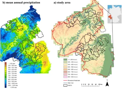
The study area consists of 53 small to medium-sized gauged catchment areas in Rhineland-Palatinate, Germany (Fig. 1a). The catchments are situated in the low mountain ranges of the Rheinisches Schiefergebirge, the Saar-Nahe-Bergland and the Rhine Valley. Most of the catchments belong to
the basins of Ahr, Wied, Lahn and Nahe, which all drain to the river Rhine. Five catchments drain directly to the Rhine. Among the 53 catchments there are 35 upstream catchments; three catchments are triple nested. The catch-ments areas vary from 9 to 1469 km2, 46 catchments areas are less than 400 km2 and 2 are larger than 1000 km2. El-evation ranges from about 100 m a.s.l. in the Rhine valley up to 818 m a.s.l. in the Hunsr¨uck, mean elevation is about 341 m a.s.l. Geology differs from schist, greywacke, and quartzite in the Rheinisches Schiefergebirge to sedimentary rock in the Saar-Nahe-Bergland and Rhine Valley. Many wa-tersheds are characterised by tertiary and quaternary volcan-ism (basaltic rocks, pumice stone and tuff).
Mean annual precipitation ranges from 530 mm yr−1in the south-east up to 1108 mm yr−1in the west and north (study period 1993–2008, Fig. 1b). Almost all watersheds are rural with little urbanization except for four catchments which are moderately urbanized (11 % to 14 %). The main land use is agricultural, but varies between 7 % and 90 % for single catchments. Some watersheds, especially in the southeast, support viticulture and orchards.
2.2 Data
For the data-driven classification method, hourly runoff and areal precipitation data for the period from January 1993 to December 2008 are available. These time series cover a wide range of diverse annual or seasonal precipitation and runoff events: from years with high precipitation and exceptionally heavy floods like 1993 or 1995 to years with very dry sum-mer periods like 2003.
Aerial precipitation was calculated with “InterMet” (Ger-lach, 2006), which interpolates meteorological data us-ing krigus-ing technique. To calculate aerial precipitation for Rhineland-Palatinate and adjacent areas, InterMet takes into account data form about 200 rain gauges, meteoro-logical data, prevailing atmospheric conditions, orography, and satellite and radar data. Typical rainfall fields extend in the range of most of the catchment sizes. In summer some mostly convective rainfall events affect only parts of catchments.
2.3 Methods
As described in the introduction, a four-step method is pur-sued for a catchment classification method. This section ex-plains the indices describing physical catchment properties and the analytical methods.
2.3.1 Event-based runoff coefficients
Fig. 1. Study area: (a) 53 catchments in Rhineland-Palatinate, Germany and (b) mean annual precipitation 1993 to 2008. Note that some
catchments are nested, so their areas overlap. Smaller catchments are plotted on top of larger ones.
significant runoff above base flow, directly following the cor-responding rainfall as given in Eq. (1).
ERC =
P
Qd Aeo· Pprec· 1000
(1) with:
ERC = Event Runoff Coefficient Qd= direct event runoff [m3h−1] Aeo= catchment area [km2]
prec = areal event precipitation [mm h−1].
The method of Merz et al. (2006) was developed for catch-ments in Austria. For this study we modified some param-eters responsible for catchment separation to optimize the method for catchments in Rhineland-Palatinate.
Comparing the resulting ERCs with manually calculated ERCs for 17 catchments in Rhineland-Palatinate verifies them. The comparison between manually and automatically calculated coefficients indicates a good fit with a mean dif-ference to all manually calculated coefficients of about 0.05. The same set of adapted criteria is used for all catchments in this study.
ERCs are calculated by a four-step approach:
a. Separation of observed runoff into baseflow and direct flow using the digital filter proposed by Chapman and Maxwell (1996).
b. Identification of peak flows, start and end of events and event-rainfall as described by Merz et al. (2006). A peak flow was identified with direct runoff twice as high as baseflow and with no larger flow 12 h before and after. To assist in event separation, a characteristic time scale of the runoff dynamics of each runoff peak was esti-mated. Start and end of an event were searched in an iterative process with the characteristic time scale and thresholds to find the time where the direct runoff at the beginning and end of an event is as small as pos-sible (Merz et al., 2006). Event rainfall was defined as the amount of rainfall within a time period before start and end of an event depending on the characteristic time scale.
c. Calculation of event runoff and rainfall volume and es-timation of ERCs following Eq. (1).
d. The calculated ERCs contain unsuitable events which are: very small events, events with insufficient data or poor event separation and events caused by snow melting.
accurately or display only low fluctuations of discharge. These exclusions affect events in summer and winter and are independent of resulting ERC.
Events caused by snow melt following a special dy-namic of runoff and do not play a major role for the response behaviour in the study area.
Unsuitable events are eliminated from the data set to improve data quality. Eliminated events with very high discharge or precipitation are checked and in case of poor separation manually calculated and saved for anal-ysis. The two events with the highest ERCs are verified by visual inspection and manual recalculation.
To represent all ERCs of one catchment, we use the Empir-ical Cumulative Distribution Function (ECDF). The ECDF is associated with the empirical measures of the sample, i.e. it estimates the true underlying distribution function of the points of a sample. Steep slopes of the ECDF indicate an independency of actual catchment conditions. Flat slopes of the ECDF indicate a high variability of ERCs influenced by actual catchment conditions.
2.3.2 Flow duration curves
For additional information about runoff behaviour concern-ing direct runoff data, we use Flow Duration Curves (FDC). The FDC is the complement of the cumulative distribution function of streamflow. In an FDC, discharge is plotted against exceedance probability and shows the percentage of time that a given flow rate is equalled or exceeded and pro-vides a probabilistic description of stream flow at a given location. A steep slope of the FDC indicates flashiness of the stream flow response to precipitation input whereas a flat-ter curve indicates a relatively damped response and a higher storage (Yadav et al., 2007).
Normalization of runoff allows for a comparison of FDC and can be done by mean (e.g. Yadav et al., 2007), by median (e.g. Clausen and Biggs, 2000) or by catchment area. Oppo-site to common daily, monthly and annual FDCs (e.g. Vogel and Fennessey, 1994; Yadav et al., 2007), we use FDCs based on hourly discharge.
2.3.3 Indices
As homogenous regions may be found for almost any set of variables (Nathan and McMahon, 1990), the selection of the most appropriate set of indices constitutes an important step. A single characteristic cannot describe all facets of catch-ment response behaviour. Therefore, we calculated a huge amount of indices which describe, seen by themselves, im-portant aspects of runoff behaviour. Indices representing ERCs are statistically derived from data of all ERCs of one catchment, again separately for summer and winter. Indices from FDCs following the “signature measures” of Yilmaz et al. (2008) describe high, medium and low flow segments of
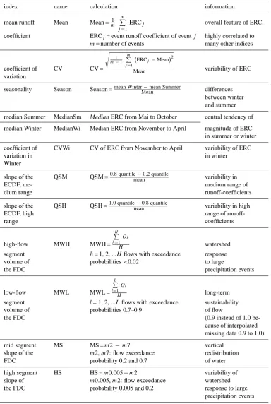
the FDCs. A correlation analysis shows very high correla-tions between many of these indices. High correlated indices (Spearman’s rho>0.8; Spearman, 1904) do not bring new in-sights into the analysis and therefore were excluded. On the other hand, we consider an even distribution of indices with respect to season, high and low flow and the importance of indices. As a result of the weighting and selection processes 12 significant indices are identified (Table 1). Six indices de-scribe mean and median ERCs, their variability and seasonal-ity and two indices characterise the mid and high segment of the ECDFs. Four indices from the FDC describe catchment behaviour of high, intermediate and low flow. The values of these 12 indices characterise the unique runoff response behaviour of one catchment.
2.3.4 SOM
The 12 indices describing catchment response behaviour of one catchment (Table 1) can be seen as a vector that spans a high-dimensional data space. The data set of each catch-ment, which is called input vector, represents the response behaviour of a catchment. For exploratory data analysis of these high-dimensional data spaces of many catchments, we use a Self-Organizing Map (SOM) which is first described 1982 by Teuvo Kohonen (Kohonen, 1982). A SOM is an un-supervised learning algorithm based on artificial neural net-works to produce a low-dimensional representation of a high-dimensional input data set. The goal of training a SOM is to present input vectors in an easily understandable form that preserves as much of the essential information in the data as possible. Kohonen (2001) provides a detailed description of the algorithm and its properties.
A SOM consists of centroids called neurons which are or-ganized on a regular grid. Each neuron is represented by a prototype vector with the same dimension as the input vectors.
There are two primary quality properties of SOM: repre-senting input data and data topology accuracy. The quality of data representation is usually measured using a quantisa-tion error defined by Euclidian distance between input vec-tors and prototype vecvec-tors. The quantisation error should be as small as possible, but there is no universal reference for it. The prototype vector with the lowest quantisation error to a certain input vector is called the Best Matching Unit (BMU) and is the basis for assigning input vectors, and thus catch-ments, to neurons. Moreover, the quantisation error of the whole SOM measures the data representation by the average Euclidian distance between input vectors and their associated BMU. The topologic error measures the topologic represen-tation: the percentage of two prototype vectors that are clos-est to a given input vector but are not neighbours on the map lattice.
Table 1. Indices describing catchment behaviour.
index name calculation information
mean runoff Mean Mean =m1
m P
j=1
ERCj overall feature of ERC,
coefficient ERCj= event runoff coefficient of eventj highly correlated to
m= number of events many other indices
coefficient of CV CV =
s
1
m−1
m
P
j=1
ERCj−Mean2
Mean variability of ERC
variation
seasonality Season Season =mean WinterMean−mean Summer differences between winter and summer
median Summer MedianSm Median ERC from Mai to October central tendency of
median Winter MedianWi Median ERC from November to April magnitude of ERC
in summer or winter
coefficient of CVWi CV of ERC from November to April variability of ERC
variation in in winter
Winter
slope of the QSM QSM =0.8 quantilemean−0.2 quantile variability in
ECDF, me- medium range of
dium range runoff-coefficients
slope of the QSH QSH =1.0 quantilemean−0.8 quantile variability in high
ECDF, high range of
runoff-range coefficients
high-flow MWH MWH =
H
P
h=1
Qh
H watershed
segment h= 1, 2, ...Hflows with exceedance response
volume of probabilities<0.02 to large
the FDC precipitation events
low-flow MWL MWL =
L
P
l=1
Ql
H long-term
segment l= 1, 2, ...Lflows with exceedance sustainability
volume of probabilities 0.7–0.9 of flow
the FDC (0.9 instead of 1.0
be-cause of interpolated missing data 0.9 to 1.0)
mid segment MS MS =m2−m7 vertical
slope of the m2,m7: flow exceedance redistribution
FDC probability 0.2 and 0.7 of water
high segment HS HS =m0.005−m2 variability of
slope of m0.005,m2: flow exceedance watershed
the FDC probability 0.005 and 0.2 response to large
manually. Small SOMs with few neurons often do not cover the complete variance of the input vectors and minimize in-terpretability; large maps perform a vague clustering.
If we want to cluster without a predefined number of clus-ters and get different levels of clustering that allow interpre-tations of cluster, we have to train a SOM with more neurons than the estimated number of clusters but small enough to define clusters. We choose the number of neurons after com-parison of differently sized SOMs to get a SOM with a rea-sonable quantisation error, no topologic error, evident levels of clustering and a high interpretability.
Prior to the SOM training, each index has to be normal-ized to ensure that all indices have equal importance inde-pendent from their values. All indices are scaled linearly so that the variance of each is equal to one. Although indices can be weighted individually, we prefer to weight all indices equally. However, the choice of indices is a kind of weight-ing in itself.
The competitive and cooperative training algorithm com-pares the Euclidean distance of an input vector to all pro-totype vectors of the SOM. Next, the neuron with the most similar prototype vector and its neighbours are adjusted to-wards the input vector. At each training step of the SOM sequential training, one input vector is chosen randomly and processed to the SOM to update the closest and nearby neu-rons. In the course of the training, the prototype vectors and their neighbours are “tuned” to all input vectors. The neu-rons of the SOM gradually specialize to represent the input and become ordered on the map lattice with nearby neurons having similar data items. The final prototype vectors form a discrete approximation of the input data distribution (Herbst et al., 2009b).
As an alternative to the sequential approach, we use the batch training algorithm of the “SOM-Toolbox for Mat-lab 5”, described in Vesanto et al. (2000), Herbst and Casper (2008) and Herbst et al. (2009b). Instead of using a single data vector at a time, the whole data set is presented to the map before any adjustments are made. In each training step, the data set is partitioned according to the Voronoi re-gions of the prototype vectors, i.e. each input vector belongs to the data set of the neuron to which it is closest. After this, the prototype vectors are updated according to the weighted average of the input samples (Vesanto et al., 2000). The batch training algorithm speeds up the training process, does not need a learning rate factor and makes the SOM independent from a random choice of dataset at start of the training, which makes a SOM reproducible.
A SOM forms a semantic map where similar samples are mapped closer together and dissimilar apart and can be used for visualizing different features. Popular visualizations of SOMs, used in this paper are:
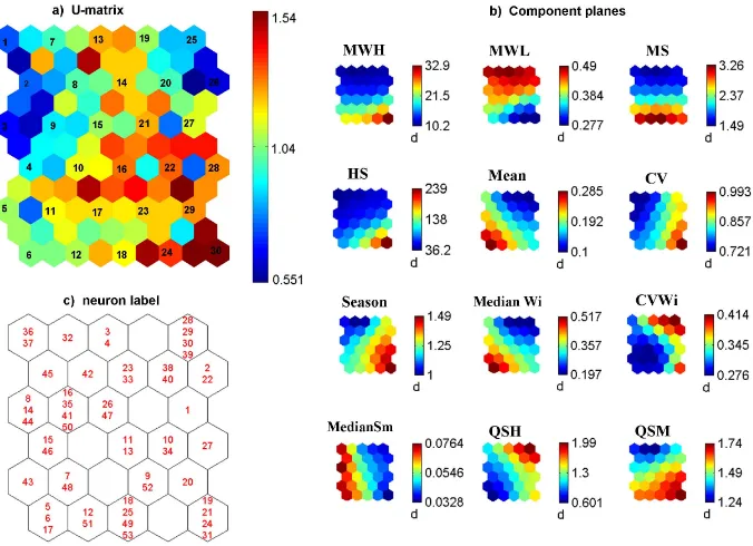
a. U-matrix (Fig. 4a): visualizes distances between two neighbouring neurons as well as the median distance from each neuron to its neighbours, and thus shows the
cluster structure of the map: high values indicate cluster borders; uniform areas of low values indicate clusters themselves.
b. Component planes (Fig. 4b): show mean values of each index onto neurons and allows recognizing separating factors between clusters.
c. Assignment of catchments to neurons (Fig. 4c): labels input vectors represented by catchment numbers to their corresponding BMU.
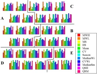
d. Distribution of index properties for each neuron (Fig. 7) demonstrated by bar charts.
All visualizations are linked by position: in each figure, a certain position corresponds to the same neuron.
2.3.5 Hierarchical clustering
Hierarchical clustering is also an unsupervised method like a SOM. In its agglomerative approach it starts with single data points as individual clusters and at each step merges the closest pair of clusters until one cluster remains. This re-quires the definition of cluster proximity. In this study we use the unweighted group average distance which defines cluster proximity as the average pairwise proximity among all pairs of points in different clusters. Usually the result is displayed as a tree-like diagram called dendrogram which displays both the cluster-subcluster relationships and the order in which the clusters were merged (Tan et al., 2006). The lengths of the limbs of the dendrogram show the proximity of cluster or points. Data items can be clustered by cutting the dendro-gram at a desired level.
3 Results
3.1 Runoff coefficients and flow duration curves
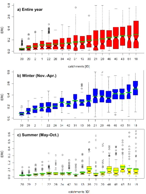
A total of 8259 Event Runoff Coefficients (ERCs) for 53 catchments were analysed, which corresponds to 100 to 200 events per watershed. There is a large variability in the ERCs. Figure 2 shows the distribution of the ERCs for 18 randomly selected catchments for a yearly (a) and sea-sonal (b and c) analysis. The 18 selected catchments repre-sent a wide range of catchment behaviour and show differ-ences of ERC between catchments. For lack of space, it is not possible to show all 53 boxplots in this figure.
b) Winter (Nov.-Apr.)
c) Summer (May-Oct.) a) Entire year
E
R
C
E
R
C
E
R
[image:8.595.49.286.59.374.2]C
Fig. 2. Boxplots of ERC for 18 catchments for (a) the entire year, (b) winter and (c) summer. The boxplots show the 25th and 75th percentile, the median, values inside the interquartile range from the box and outliers of the event runoff coefficients. The green lines indicate the mean ERC. The widths of the boxes are propor-tional to the square-roots of the number of ERCs for this catchment.
some single summer events with larger ERCs occur in each catchment.
These outliers are caused by intensive convective precipi-tation events often in combination with heavy thunderstorms. Variability of ERCs tend to be larger in winter than in sum-mer, but most catchments show less skewed distributions and relative short boxes which indicate the 25th and 75th per-centiles in Fig. 2b. Thus, during winter, 50 % of the events of a catchment reach an analogous ERC, whereas the other 50 % display a much higher variability.
Event durations are between less than one day and many days.
The Empirical Distribution Functions (ECDFs) in Fig. 3a display the distribution of ERCs for each catchment. The lower part of the ECDFs is dominated by very low ERC that occur in summer. The ECDFs show characteristic shapes for each catchment.
To compare the FDCs of different catchments by their re-sponse behaviour we have to normalize them in a way that influences of physiogeographic and hydroclimatic conditions
are mostly excluded. Normalization by catchment area shows high influences of mean annual precipitation and is therefore not suitable for this study. Normalization by mean results in FDCs not well distinguishable for low exceedance probabilities and shows a high dependence of extreme val-ues, covered by other indices in this study. Therefore, runoff for FDCs is normalized by its median value (Q.5) to elim-inate most of the influences of mean annual precipitation, catchment area and extreme high or low flow and get well distinguishable FDCs. The FDC (Fig. 3b) show a wide range of runoff behaviour in all segments from flat curves to steep curves. Moreover, even in the geographically restricted re-gion which includes nested catchments there are quite dif-ferent response characteristics suitable for comparison and clustering.
3.2 Clustering by catchment response behaviour
In this paper two or more catchments are assumed to be-have similar if similarity in the ECDFs and FDCs are given. Catchments with similar response behaviour are grouped by training a SOM and implementing hierarchical clustering on the SOM.
The dimension of the SOM is manually adjusted to 30 neu-rons on a 5×6 grid. This dimension has optimal explanatory power of the U-matrix (Fig. 4a) and a topological error of zero.
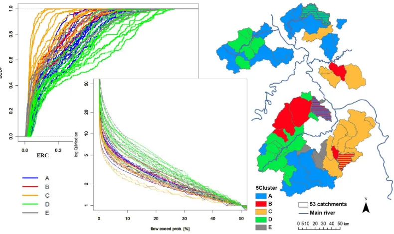
The SOM grid with the assignment of 53 available catch-ments to neurons (Fig. 4c) shows 25 neurons labelled with up to four catchment numbers. Catchments that are labelled to-gether on one neuron can be considered as behaving similar and build the smallest unit of clustering. SOM reduces the variability of 53 catchments to 25 neurons. To further reduce the number of groups we apply a cluster analysis. The U-matrix (Fig. 4a) shows obviously different parts of the map: two blue-coloured regions in the upper part indicate units with a high degree of similarity, which can be seen as sep-arate clusters. A row of red and orange colours sepsep-arates the two bottom rows of neurons from the remaining map and builds a cluster border. Further visual clustering or setting of cluster borders is difficult. Therefore, we perform hierarchi-cal clustering on the SOM. The dendrogram (Fig. 5) shows the arrangement of five reasonable clusters, which are named with capital letters A to E. The transfer of the cluster from the dendrogram to the U-matrix of the SOM is displayed in Fig. 5 as well. With the help of the assignment of catch-ments to neurons (Fig. 4c) we can relate catchcatch-ments to the clustering. Despite overlapping ECDFs and FDCs (Fig. 6), the clusters are clearly visible in both diagrams. The spatial distribution of clustered catchments (Fig. 6) shows a group-ing of catchments with similar response behaviour, but also some catchments which do not belong to a group.
a) b)
Fig. 3. Catchments response behaviour of 53 catchments for the entire year: (a) empirical cumulative distribution functions of event runoff
coefficients and (b) flow duration curves, normalized by median.
Fig. 4. Visualizations of a SOM: (a) unified distance matrix: neurons of the SOM are indicated by numbers. It shows structures by
visualising distances between neighbouring neurons and, on additional hexagons between neurons, median distances between two neurons.
(b) Component planes for each index display mean values of each index on the neurons of the SOM. (c) Assignment of catchments to neurons
labels catchment IDs to their corresponding BMU1. All visualizations of SOMs are linked by position: in each figure, a certain position corresponds to the same neuron.
quantisation errors less than 2.7, 58 % are below 1.6. For comparison: the general quantisation error is 1.64. But four catchment data sets have very high quantisation errors be-tween 2.98 and 4.43. These catchments (3, 4, 21 and 31), labelled to neurons at the edge of the SOM, can be consid-ered having special response behaviour, not very well cov-ered by the SOM. They display extreme values for most of
[image:9.595.130.468.299.544.2]1
a
4 3
2
5 1
8
9
10 13
11 17 14
15
16
12 18 19
20
22 21
23
24 25
26
28
29
30 6
7
27
A
E
D
B
C
B
[image:10.595.128.468.64.210.2]C
A
D
E
Fig. 5. Dendrogram on SOM and U-matrix with cluster. Numbers in the dendrogram correspond to neuron numbers on the U-matrix; capital
letters indicate clusters.
Fig. 6. Clusters by catchment response behaviour: empirical distribution function of event runoff coefficients, flow duration curve (limb<50 %) and spatial distribution. The striped catchments in the map are borderline cases, shown in colours of their first and second best cluster. Note, some catchments are nested, so their areas overlap. Smaller catchments are plotted on top of larger ones.
low values of one or more characteristic aspect of runoff re-sponse, which makes them distinguishable from each other. This discernibility is a clear indication of the potential of the SOM to build classes of similar behaviour. Cluster B shows a medium response behaviour indicated by medium values of all indices. These clusters will be discussed and interpreted together with physical catchment properties in Sect. 3.4 (Comparison).
A possible disadvantage to our and many other methods of classification is the certainty of the allocation of catch-ments to a particular class. Classes of similar catchcatch-ments by response behaviour or by physical catchment characteris-tics do not show sharp borders, especially for catchments in
[image:10.595.101.496.260.495.2]Fig. 7. Distribution of index properties for each neuron as bar charts. Lines indicate cluster border, letters cluster names.
Table 2. Characteristics of cluster A to E by catchment response
behaviour.
characteristic
cluster runoff variability seasonality reactivity coefficients runoff runoff runoff
coefficients coefficients
A ∼ – – –
summer:+
B −− + + −−
C – ∼ −− –
winter++
D ++ −− −− +
E + ++ ++ ++
summer:–
with: ++ very high, + high,∼medium,−−low, – very low
borderline catchments we use their quantisation errors to the BMU and to the neuron of the neighbouring cluster. Catch-ments with a similar quantisation error to different neurons can be recognized as belonging to two neurons and thus may belong to two clusters. With this procedure, we can im-prove clustering and areal grouping of catchments (Fig. 6). We can identify three borderline cases (catchments 1, 26 and 43) from the clusters by response behaviour. They belong to neurons at the edge of a cluster with medium distance to a neighbouring neuron of another cluster. In their first 6 BMUs
there is a frequent change between both clusters with slightly increasing quantisation errors. Therefore, we assign them to both clusters: catchment 1 to B and C, catchment 26 to A and B and catchment 43 to D and A.
3.3 Physical catchment properties
A list of physical catchment properties is compiled from a digital elevation model and different digital sources that de-scribe catchment size, flow length, drainage density, topog-raphy, geology, soils, land use and climate of the catchments. All of them have more or less impact on runoff.
Yadav et al. (2007) recognised that using too many dy-namical properties simultaneously often results in a rejec-tion of all models, which is also our experience. Further-more, different degrees of influence make it necessary to weight and choose certain groups of catchment characteris-tics. To reduce this amount of indices and to avoid redun-dancies, we eliminate all indices with high correlation co-efficients (Spearman’s rho >0.8; Spearman 1904) to other indices. From the remaining indices, we choose indices with high correlation to indices of runoff behaviour considering physical indices identified in other studies as most important for runoff behaviour.
[image:11.595.58.280.404.552.2]from the flow duration curve. Correlation coefficients be-tween catchment size and the other indices are consider-ably lower. Within the 46 catchments (87 %) smaller than 370 km2, correlation coefficients show no correlation be-tween catchment size and the chosen runoff indices. Also Merz and Bl¨oschl (2009) found no correlation of mean event runoff coefficients and their variability to catchment size for catchments in Austria. Yadav et al. (2007) suggest that catch-ment area isn’t the most important physical characteristic de-scribing response behaviour for English catchments.
The result of the selection process to find responsible catchment attributes for the study region are six meaningful catchment properties:
– Mean Annual Precipitation 1993–2008 (MAP),
– mean long-term potential evaporation (ET), calculated from raster data of the mean annual potential grass ref-erence evapotranspiration from the “Hydrological Atlas of Germany” for the period from 1961 to 1990 (Bun-desministerium f¨ur Umwelt, Naturschutz und Reaktor-sicherheit, 2000),
– Wetness index: ratio of MAP to ET (Wet),
– mean slope derived from a digital elevation model with a resolution of 20 m (Slope),
– average field capacity derived from Boden¨ubersichts-karte 1:200 000 von Rheinland-Pfalz (B ¨UK 200) (FK), – percentage of area with intense to medium ground
water recharge, derived from Hydrologischer Atlas Rheinland-Pfalz and Geologische ¨Ubersichtskarte von Rheinland- Pfalz 1:300 000 (GUEK 300) (GW). Climate and antecedent soil moisture are suggested as a ma-jor control in runoff generation (Sankarasubramanian and Vogel, 2002; Yadav et al., 2007; Merz and Bl¨oschl, 2009). Therefore, half of the used indices describe climate. The wetness index as an expression of long-term water balance is highly correlated with MAP. Using MAP and the wetness index can also be seen as a weighting of MAP as the most important catchment property.
The spatial arrangement of clusters by behaviour (Fig. 6) follows a simplified gradient of increasing mean annual pre-cipitation (MAP) from East to West and South to North. There is a high correlation between MAP and mean ERCs with a trend of increasing mean ERCs with increasing MAP. With increasing MAP, it becomes more likely that initial con-ditions are wet, thus enhancing runoff generation. The sea-sonal variability of ERCs (Fig. 2) reveals the changes in an-tecedent soil moisture and evapotranspiration. Climate has the largest influence on runoff behaviour not least by influ-encing drainage characteristics, controlling geomorpholog-ical structures, soils and vegetation (Sivapalan, 2005; Nor-biato et al., 2009).
Pfister et al. (2002) and Hellebrand et al. (2007) found a strong relationship between winter storm flow coefficients and the permeability of the substratum for catchments in the Grand Duchy of Luxembourg and Rhineland-Palatinate which is represented here by the average field capacity and the ground water recharge.
Other catchment properties like flow length, catchment size, slope heterogeneity or land use show no important in-fluence on the chosen indices of runoff behaviour or are elim-inated because of high correlation to included indices.
Note, that because of not available data for all catchments, clustering of catchments by physical properties and compar-ison of catchments (Sect. 3.4) is based on 45 catchments.
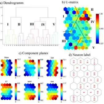
Training a SOM with 4×7 neurons and performing hi-erarchical clustering on the SOM, the same method as used before, lead to 5 reasonable clusters of catchment properties (Fig. 8). The SOM grid with the labelled neurons (Fig. 8d) shows a clustering of the 45 catchments on 22 neurons. There are up to 4 catchments labelled on one neuron, building the smallest unit of clustering. The dendrogram (Fig. 8a) justifies the choice of five clusters, which are named with roman nu-merals I to V. With the help of the labelled neurons (Fig. 8d) and the component planes (Fig. 8c), we characterise these clusters as described in Sect. 3.4 (comparison).
Within the clusters by physical catchment properties we identify 5 borderline catchments: 1, B and C; 26, A and B; 27, B and E; 39, C and B; 43, D and A.
3.4 Comparison
The spatial variability of catchment response behaviour is supposed to be dependent on its physiographic and climatic characteristics. Following this a priori assumption, we search for corresponding clusters of catchments with similar phys-ical catchment characteristics to illustrate the plausibility of the classification by response behaviour.
For each cluster of catchment behaviour, we counted the number of catchments matching a certain cluster of catch-ment properties (Table 3). Corresponding clusters show the highest overlap of catchments (Table 3, yellow). For most of the clusters, the number of shared basins allows a clear as-signment. Only catchments from clusters B and IV cannot be clearly assigned to a corresponding cluster. Furthermore, clusters B and IV both represent medium response behaviour and medium catchment properties, i.e. they show reasonable corresponding catchment properties. Therefore, we assign cluster B to cluster IV. Attaching borderline catchments to their second best cluster (Table 3) supports the assignment B to IV.
Fig. 8. SOM and clusters by physical catchment properties. (a) Dendrogram of SOM indicates cluster I to V, (b) unified distance matrix
with neurons indicated by numbers and clusters; shows structures by visualising distances between neighbouring neurons and, on additional hexagons, median distances between two neurons. (c) Component planes for each index display mean values of the index onto the neurons of the SOM. (d) Assignment of catchments to neurons labels catchment IDs to their corresponding BMU1. In each figure, a certain position corresponds to the same neuron.
study area with 893 catchments is much larger than ours. This may indicate a possibility for classification and accom-panying problems across scales.
Corresponding clusters show appropriate catchment prop-erties (clusters I to V) and catchment response behaviour (clusters A to E):
– I: Very steep catchments with low water storage capac-ity, low MAP and high ET; it correspond to E with high ERCs and very high variability, seasonality and reactivity.
– II: Low slopes, high water storage capacity but dry with high ET; corresponds to C with very low ERCs and reactivity, low seasonality and medium variability but high variability in winter.
– III: High mean slopes, very low water storage capaci-ties, high MAP and low to medium ET; it correspond to two quite different clusters: A and D. With these
catchment properties one would expect high ERCs and reactivity and low variability and seasonality – as in cluster D, not cluster A. In this case we can assume a lack of important physical characteristics in the analy-sis. Most of the catchments of cluster A are larger, shal-lower, have larger flow lengths, larger drainage density and have more agriculturally used areas and less forests than catchments of cluster D.
– IV: No exceptional values at all; it corresponds to B. Both clusters show medium values for all aspects of response behaviour as well as of physical catchment characteristics.
Table 3. Overlap between clusters of response behaviour (A to E)
and clusters of catchment properties (I to V). Numbers indicate the number of corresponding catchments. Numbers in brackets indi-cate the number of corresponding catchments considering border-line catchments assigned to their second best cluster. Correspond-ing clusters are marked in yellow.
response behaviour
A B C D E
catchment properties
I 1 (1) 3 (1) 5 (5)
II 1 (−) 5 (8)
III 6 (7) 2 (2) 7 (8)
IV 3 (−) 2 (3) 2 (2) 2 (1)
V 5 (7) 1 (−)
4 Discussion
Although the study area is comparatively small and homo-geneous and there are many nested catchments, the indices describing catchment response behaviour show a high dis-criminating power and enable us to characterise catchments. Clustering of catchments by their response behaviour as well as by their physical properties leads to five clusters, each rep-resenting different facets of flow regimes or types of catch-ments. The comparison of the two pools of clusters show plausible classes of catchments. Each class of response be-haviour represents different facets of flow regimes and can be characterised by high or low values of special aspects of re-sponse behaviour. Two classes are determined by steep flow duration curves and by the highest ERCs. This behaviour corresponds with steep catchment slopes and low water stor-age capacities. Different mean annual precipitation causes corresponding higher or lower runoff coefficients. Catch-ments with flatter flow duration curves display the lowest runoff coefficients. Moreover, due to their higher water stor-age capacities low seasonality and variability of ERCs are apparent. Within this group of catchments, differences in mean annual precipitation and potential evapotranspiration cause different runoff coefficients.
The comparison of clusters based on (i) response be-haviour and (ii) physical catchment properties can be seen as a review of interpretability of the clustering by response behaviour. It allows connecting catchment behaviour with physical catchment properties as a basis for catchment clas-sification covering both kinds of catchment characteristics. Most of the catchment characteristics, which are obtained by the classification method, can be interpreted well.
In Sect. 3.2, we define borderline catchments as catch-ments on the border of two clusters, near the overlap. We
can identify 3 borderline catchments in the clusters based on runoff behaviour and 5 borderline cases in the clusters based on physical catchment properties. If we assign these 8 bor-derline catchments to their second best cluster, we improve the overlap between the two pools of clusters from 67 % to 84 % (Table 3).
Thus, we divide the classified catchments into three groups:
1. catchments within the overlap: catchment behaviour is closely related to the considered physical catchment properties,
2. catchments near the overlap: catchment behaviour is re-lated to the considered catchment properties and addi-tional property(s),
3. catchments outside the overlap: individual physical catchment properties are responsible for catchment re-sponse behaviour.
The Classification of catchments in group (1) is clear. For the classification of catchments in group (2), we may define a differing class taking into account additional facts. Catch-ments of group (3) represent a subclass which is caused by special catchment properties. This subclass of catchments with similar behaviour but different physical catchment prop-erties describes a so called “process equifinality” in the runoff signal (Hellebrand et al., 2011). Different processes producing the same values of discharge characteristics in dif-ferent basins. For example, catchment 28 (Planig, 171 km2) fits well to clusters C and II, like most catchments from clus-ter C; catchment 39 (Schulm¨uhle, 145 km2) belongs to clus-ter C too but fits to clusclus-ter IV. None of these catchments are borderline cases, both show very low to medium quantisa-tion errors to their BMUs. The indices of both catchments are inside the range of indices of cluster C, they can be as-sumed to as behave similarly. On the U-matrix (Fig. 8b), clusters II and IV are neighbouring clusters but well sepa-rated by a row of neurons indicating high differences, show-ing a clear separation of both clusters. This case of process equifinality points to different processes but similar runoff behaviour and can be figured out by comparing both pools of clusters.
5 Conclusions
In this study, we define each five distinguishable classes of catchment behaviour and physical catchment properties by using SOMs. The comparison of the two pools of clusters, show a high overlap between both cluster sets. We take this as a sign that SOM has detected well structures inherent the catchment behaviour.
The SOM serves as a tool for unsupervised clustering, but also to analyse and visualize the clusters itself. In spite of using a default dimension of the SOM we train a SOM with 30 neurons, which is the optimal SOM dimension for the used data set. For other data sets, the optimal dimension of a SOM has to be found in an iterative process. Here, the large number of neurons makes hierarchical clustering on the SOM necessary to define cluster borders. On the other hand, a large number of neurons in combination with the topolog-ical correctness of SOMs offer a scope of interpretation of the clusters itself and their relationships, to find catchments with extreme response behaviour or to identify and discuss borderline cluster to improve clustering. Visualizations like the bar charts with index properties for each neuron in Fig. 7 or component planes in Fig. 4b describe clusters and iden-tify indices causes clustering. Furthermore, SOMs allow to project any data set with the same dimensionality outside the training data set onto the map and thus to a certain cluster. Therefore a SOM can be used as a tool for classification of (new) data sets.
The presented approach allows the identification of clus-ters of similar catchment response behaviour and next, to classify catchments by their response behaviour with a view to physical catchment properties. A comparison with catch-ments clustered by physical properties shows a reasonable overlap which can be improved by analysis of SOMs. Still, a number of catchments show individual runoff response be-haviour which cannot be explained by catchments proper-ties considered here. The individuality of catchments limits the possibilities of simplifying runoff generation. To find a meaningful classification of catchments, both kinds of catch-ment characteristics have to be taken into account.
The classification presented in this study is valid for catch-ments in the study area in Rhineland-Palatinate. Catchcatch-ments in other landscapes or at other scales may have other classi-fication items because of influence, different processes have on the runoff response. However, the methodology presented in this paper is independent of landscape and scale.
Acknowledgements. This investigation was carried out within the
Research Center for Regional and Environmental Statistics (Forum-Stat) at the University of Trier, financed by the Research-Initiative Rhineland-Palatinate. The authors wish to thank the State Office for Environment, Water Management and Trade Control (LUWG) Rhineland-Palatinate at Mainz for providing data of runoff and pcipitation. We would like to thank Uwe Ehret, two anonymous re-viewers and the editor Attilio Castellarin for their constructive com-ments that greatly helped improving this paper.
Edited by: A. Castellarin
References
Acreman, M. C. and Sinclair, C. D.: Classification of drainage basins according to their physical characteristics: an application for flood frequency analysis in Scotland, J. Hydrol., 84, 365–380, 1986.
Beven, K. J.: Uniqueness of place and process representations in hydrological modelling, Hydrol. Earth Syst. Sci., 4, 203–213, doi:10.5194/hess-4-203-2000, 2000.
Blume, T., Zehe, E., and Bronstert, A.: Rainfall-runoff response, event-based runoff coefficients and hydrograph separation, Hy-drolog. Sci. J., 52, 843–862, 2007.
Bundesministerium f¨ur Umwelt: Naturschutz und Reaktorsicher-heit (Hrsg), Hydrologischer Atlas von Deutschland, 2000. Burn, D. H.: Catchment similarity for regional flood frequency
analysis using seasonality measures, J. Hydrol., 202, 212–230, 1997.
Chapman, T. G. and Maxwell, A. I.: Baseflow Separation – Com-parison of Numerical Methods with Tracer Experiments, I. E. Aust. Natl. conf. Publ. 96/05, 539–545, 1996.
Clausen, B. and Biggs, B. J. F.: Flow variables for ecological studies in temperate streams: grouping based on covariance, J. Hydrol., 237, 184–197, 2000.
Di Prinzio, M., Castellarin, A., and Toth, E.: Data-driven catch-ment classification: application to the pub problem, Hydrol. Earth Syst. Sci., 15, 1921–1935, doi:10.5194/hess-15-1921-2011, 2011.
Gerlach, N.: INTERMET – Interpolation meteorologischer Gr¨oßen, Veranstaltungen 3/2006 – Niederschlag-Abfluss-Modellierung zur Verl¨angerung des Vorhersagezeitraumes operationeller Wasserstands- und Abflussvorhersagen, Kollo-quium am 27 Sepember 2005 in Koblenz, Bundesanstalt f¨ur Gew¨asserkunde, 2006.
Hall, M. and Minns, A.: The classification of hydrologically homo-geneous regions, Hydrolog. Sci. J., 44, 693–704, 1999.
Hellebrand, H., Hoffmann, L., Juilleret, J., and Pfister, L.: Assess-ing winter storm flow generation by means of permeability of the lithology and dominating runoff production processes, Hy-drol. Earth Syst. Sci., 11, 1673–1682, doi:10.5194/hess-11-1673-2007, 2007.
Hellebrand, H., M¨uller, C., Fenicia, F., Matgen, P., and Savenije, H.: A process proof test for model concepts: modelling the meso-scale, Phys. Chem. Earth, 36, 42–53, 2011.
Herbst, M. and Casper, M. C.: Towards model evaluation and iden-tification using Self-Organizing Maps, Hydrol. Earth Syst. Sci., 12, 657–667, doi:10.5194/hess-12-657-2008, 2008.
Herbst, M., Gupta, H. V., and Casper, M. C.: Mapping model be-haviour using Self-Organizing Maps, Hydrol. Earth Syst. Sci., 13, 395–409, doi:10.5194/hess-13-395-2009, 2009a.
Herbst, M., Casper, M. C., Grundmann, J., and Buchholz, O.: Com-parative analysis of model behaviour for flood prediction pur-poses using Self-Organizing Maps, Nat. Hazards Earth Syst. Sci., 9, 373–392, doi:10.5194/nhess-9-373-2009, 2009b.
Kaski, S.: Data Exploration Using Self-Organizing Maps, Dr. the-sis, Department of Computer Science and Engineering, Helsinki University of Technology, Helsinki, 57 pp., 1997.
Kohonen, T.: Self-Organize Formation of Topologically Correct Feature Maps, Biol. Cybern., 43, 59–69, 1982.
Kohonen, T.: Self-Organizing Maps, 3rd Edn., Information Sci-ences, Springer, Berlin, Heidelberg, New York, 501 pp., 2001. Maimon, O. and Rokach, L.: Data mining and knowledge discovery
handbook, Springer, New York, 1383 pp., 2005.
McDonnell, J. J. and Woods, R.: On the need for catchment classi-fication, J. Hydrol., 299, 2–3, 2004.
Merz, R. and Bl¨oschl, G.: A process typology of regional floods, Water Resour. Res., 39, 1340, doi:10.1029/2002WR001952, 2003.
Merz, R., Bl¨oschl, G., and Parajka, J.: Spatio-temporal variability of event runoff coefficients, J. Hydrol., 331, 591–604, 2006. Merz, R. and Bl¨oschl, G.: A regional analysis of event
runoff coefficients with respect to climate and catchment characteristics in Austria, Water Resour. Res., 45, W01405, doi:10.1029/2008WR007163, 2009.
Nathan, R. J. and McMahon, T. A.: Identification of homogenous regions for the purposes of regionalisation, J. Hydrol., 121, 217– 218, 1990.
Norbiato, D., Borga, M., Merz, R., Bl¨oschl, G., and Carton, A.: Controls on event runoff coefficients in the eastern Italian Alps, J. Hydrol., 375, 312–325, 2009.
Oudin, L., Kay, A., Andr´eassian, V., and Perrin, C.: Are seemingly physically similar catchments truly hydrologically similar?, Wa-ter Resour. Res., 46, W11558, doi:10.1029/2009WR008887, 2010.
Pfister, L., Iffly, J.-F., and Hoffmann, L.: Use of regionalized storm-flow coefficients with a view to hydroclimatological hazard map-ping, Hydrolog. Sci. J., 47, 479–492, 2002.
Ramachandra Rao, A. and Srinivas, V. V.: Regionalization of wa-tersheds, An Aproach based on Cluster Analysis, Springer Sci-ence + Business Media B. V., 2008.
Sankarasubramanian, A. and Vogel, R. M.: Annual hydroclima-tology of the United States, Water Resour. Res., 38, 1–12, doi:10.1029/2001WR000619, 2002.
Sivapalan, M., Takeuchi, K., Franks, S. W., Gupta, V. K., Karam-biri, H., Lakshmi, V., Liang, X., McDonell, J. J., Mendiondo, E. M., O’Connell, P. E., Oki, T., Pomeroy, J. W., Schertzer, D., Uh-lenbrook, S., and Zehe, E.: IAHS Decade on Predictions in Un-gauged Basins (PUB), 2003–2012: Shaping an exciting future for the hydrological sciences, Hydrolog. Sci. J., 48, 857–880, doi:10.1623/hysj.48.6.857.51421, 2003.
Sivapalan, M.: Pattern, Process and Function: Elements of a Uni-fied Theory of Hydrology at the CatchmentScale, in: Ency-clopaedia of hydrological sciences, edited by: Anderson, M., John Wiley, London, 193–219, 2005.
Spearman, C.: The Proof and Measurement of Association between Two Things, Am. J. Psychol., 15, 72–101, 1904.
Stedinger, J. R., Vogel, R. M., and Foufoula-Georgiou, E.: Fre-quency analysis of extreme events, in: Handbook of Hydrology, edited by: Maidment, D. R., McGraw-Hill, New York, p.18.35, 1992.
Tan, P.-N., Steinbach, M., and Kumar, V.: Introduction to Data Min-ing, Pearson Education, Addison Wesley, Boston, 769 pp., 2006. Toth, E.: Classification of hydro-meteorological conditions and multiple artificial neural networks for streamflow forecasting, Hydrol. Earth Syst. Sci., 13, 1555–1566, doi:10.5194/hess-13-1555-2009, 2009.
van Dijk, A. I. J. M.: Climate and terrain factors explaining stream-flow response and recession in Australian catchments, Hydrol. Earth Syst. Sci., 14, 159–169, doi:10.5194/hess-14-159-2010, 2010.
Vesanto, J., Himgerg, J., Alhoniemi, E., and Parhankangas, J.: SOM Toolbox for Matlab 5, Helsinki University of Technology, Re-port A59, Espoo, Finland, 60 pp., 2000.
Vogel, R. M. and Fennesey, N. M.: Flow Duration Curves I: New Interpretation and Confidence Intervals, J. Water Res. Pl.-ASCE, 120, 485–504, 1994.
Wagener, T., Sivapalan, M., Troch, P. and Woods R.: Catchment Classification and Hydrologic Similarity, Geography Compass, 1/4, 901–931, 2007.
Woods, R.: Seeing catchments with new eyes, Hydrol. Process., 16, 1111–1113, 2002.
Yadav, M., Wagener, T., and Gupta, H.: Regionalization of con-straints on expected watershed response behavior for improved predictions in ungauged basins, Adv. Water Resour., 30, 1765– 1774, 2007.