Parameterization of a bucket model for soil vegetation atmosphere modeling under seasonal climatic regimes

www.hydrol-earth-syst-sci.net/15/3877/2011/ doi:10.5194/hess-15-3877-2011

© Author(s) 2011. CC Attribution 3.0 License.

Earth System

Sciences

Parameterization of a bucket model for soil-vegetation-atmosphere

modeling under seasonal climatic regimes

N. Romano, M. Palladino, and G. B. Chirico

Department of Agricultural Engineering and Agronomy, University of Napoli Federico II, Portici (Napoli), Italy Received: 15 May 2011 – Published in Hydrol. Earth Syst. Sci. Discuss.: 24 May 2011

Revised: 24 November 2011 – Accepted: 25 November 2011 – Published: 21 December 2011

Abstract. We investigate the potential impact of account-ing for seasonal variations in the climatic forcaccount-ing and usaccount-ing different methods to parameterize the soil water content at field capacity on the water balance components computed by a bucket model (BM). The single-layer BM of Guswa et al. (2002) is employed, whereas the Richards equation (RE) based Soil Water Atmosphere Plant (SWAP) model is used as a benchmark model. The results are analyzed for two differently-textured soils and for some synthetic runs under real-like seasonal weather conditions, using stochastically-generated daily rainfall data for a period of 100 years. Since transient soil-moisture dynamics and climatic seasonality play a key role in certain zones of the World, such as in Mediterranean land areas, a specific feature of this study is to test the prediction capability of the bucket model under a condition where seasonal variations in rainfall are not in phase with the variations in plant transpiration. Reference is made to a hydrologic year in which we have a rainy period (starting 1 November and lasting 151 days) where vegetation is basically assumed in a dormant stage, followed by a drier and rainless period with a vegetation regrowth phase. Bet-ter agreement between BM and RE-SWAP inBet-tercomparison results are obtained when BM is parameterized by a field ca-pacity value determined through the drainage method pro-posed by Romano and Santini (2002). Depending on the vegetation regrowth or dormant seasons, rainfall variability within a season results in transpiration regimes and soil mois-ture fluctuations with distinctive feamois-tures. During the vege-tation regrowth season, transpiration exerts a key control on soil water budget with respect to rainfall. During the dormant season of vegetation, the precipitation regime becomes an important climate forcing. Simulations also highlight the oc-currence of bimodality in the probability distribution of soil

Correspondence to: N. Romano ([email protected])

moisture during the season when plants are dormant, reflect-ing that soil, it bereflect-ing of coarser or finer texture, can be pref-erentially in either wetter or drier states over this period.

1 Introduction

Progress has been achieved in advancing scientific knowl-edge on the interactions within the soil-vegetation-atmosphere (SVA) system and also in developing improved monitoring and modeling technologies. However, there is still little information transferred from the research world to the tools used by public agencies, consultants, and stakehold-ers responsible for managing land and water resources. On the one hand, hydrologic models developed by scientists are usually very complex and require large amounts of special-ized input data that may not be directly available (H¨ollander et al., 2009). On the other hand, simple models are easy to use, but may be of inadequate accuracy or detail to answer specific management questions, especially in cases of multi-ple demands upon the SVA system.

accurately most of practical soil-water flow problems (Ro-mano et al., 1998; ˇSim˚unek et al., 2008). Employing RE at laboratory soil core or field plot scales can be done with con-fidence (Sposito, 1986), but may become unmanageable for hydrologic applications at the scales of hillslopes and catch-ments chiefly because of the spatial, and sometimes also tem-poral, variability exhibited by the soil hydraulic properties (Sharma and Luxmoore, 1979; Braud, 1998; Settin et al., 2007), and partly because of theoretical doubts that capillary suction heads and hydraulic gradients are still the driving forces of mass flow and momentum transfer in unsaturated porous media at such larger scales (Beven, 1989; McDonnell et al., 2007). Notwithstanding these limitations, RE is in-creasingly being used in process-based distributed models of hydrological cycle and is also used at the global scale in Land Surface Models (Kowalczyk et al., 2006; Clark et al., 2008; Manus et al., 2009; Oleson et al., 2010). Moreover, RE so-lutions are anyhow considered as the best available reference for comparisons to the performances of simplified models to be categorized in terms of their complexity with respect to the number of hydrologic processes employed (Guswa et al., 2002).

The soil water balance bucket model (BM) of Manabe (1969) is the classic example of a lumped model accounting for a simplified description of the major processes evolving in the hydrologic cycle, in which a single soil layer is concep-tualized as a bucket receiving and retaining all incident water until its storage capacity is filled. The latter assumption, for example, saves one the need of describing infiltration rate with respect to rainfall intensity through an analytical (usu-ally, empirical) equation. This type of model is particularly efficient to describe land surface processes and thus exten-sively used when coupled with large scale atmospheric mod-els, including General Circulation Models (GCMs), but may experience problems due to its simple representation of veg-etation and estimation of potential evapotranspiration fluxes (Seneviratne et al., 2010). Since the valuable function of soil to transfer water with different rates along the vertical profile is virtually ignored and a direct feedback is described be-tween soil water storage and evapotranspiration, BM is char-acterized by a rather short soil water storage memory and can hardly describe correctly the system response to rapid time evolution in atmospheric forcing. Yet, in the last decades sev-eral studies have shown that bucket models can be efficiently employed for predicting some components of the soil water budget, as they provide results similar to those observed in the field or those simulated with models which are more de-tailed in the description of the soil water dynamics, at least in soils with specific climatic regimes (Milly, 1994; Guswa et al., 2002; Farmer et al., 2003).

On the wave of studies gaining insights into the poten-tial impacts that land use and climate changes may exert on catchment scale hydrologic response, one challenging ques-tion is to obtain efficient predicques-tions while recognizing that water transfer in the SVA continuum is controlled by several

non-linear and dynamic interacting processes (Bl¨oschl and Montanari, 2010). The efficiency of simplified models has been tested in areas characterized by stationary condition of the climatic forcing (Milly et al., 2008), which can be ob-served only in limited zones of the World, such as in the sa-vannas of South Africa (Porporato et al., 2002). Instead, tran-sient soil-moisture dynamics and climatic seasonality play a key role in other environments (Settin et al., 2007), such as those characterized by Mediterranean climates, where rain-fall shows an out-of-phase relationship with air temperature, with an alternation of wet-cold and dry-warm periods. The end of wet-cold period corresponds to the beginning of the growing season, when water dynamics are mainly controlled by the evapotranspiration processes, which induce a progres-sive reduction of the water stored toward the dry-warm sea-son. The soil-moisture dynamics during the growing season is generally far from what can be predicted with the hypothe-sis of stationarity. Nevertheless, under such complex climatic variability during the year, linking the fluxes and vegetation growth to the variations in soil water contents along the en-tire soil profile can be a prerequisite to adequately simulate fluctuations in evapotranspiration or other hydrologic fluxes. A general objective of the present work is to assess the validity of using a bucket model to simulate the local water balance and associated fluxes assuming a rainfall regime and vegetation characteristics representative of Mediterranean ar-eas. Comparisons are carried out with respect to the re-sults obtained under the same conditions through a RE-based hydrologic model. Under climate, vegetation, and soil conditions relevant to an African savannah site, Guswa et al. (2002) have shown that an appropriate formulation of the single-layer bucket model, with proper account of the rela-tionship between transpiration,T, and degree of saturation in soil,s, can provide results similar to those obtained by a more comprehensive model based on the integration of the verti-cally discretized Richards equation. At relatively larger time-scale, namely an entire growing season of 200 days, Table 5 of this paper reports some more similarity among the wa-ter fluxes as computed by the RE or BM models. However, when moving to a smaller scale, namely the daily time-scale, discrepancies between RE model results and those of the BM of Guswa et al. (2002) were about 50 % for evap-otranspiration flux, ET, and ranged from 50 % to 70 % over a season for theT/ET ratio (see, for example, the traces of daily transpiration depicted in Fig. 8 of that paper).

field capacity, then this excess of water is routed to runoff only, or to both runoff and drainage. Notwithstanding the considerable importance of field capacity in a bucket-type hydrologic approach, its value is still determined using sim-plified, often very inaccurate techniques (Romano and San-tini, 2002). In view of parameterizing a bucket model for effectively computing the soil water budget under environ-mental conditions representative of a Mediterranean area, a specific objective of this study is to evaluate whether the de-termination of the field capacity value with an appropriate technique can lead to BM results more in agreement with those offered by a more complex model based on RE.

2 Description of the models

2.1 The SWAP model

SWAP (Soil, Water, Atmosphere and Plant) is a widespread used model in the soil hydrology community to simulate soil water flow in the vadose zone at field scale and during entire growing seasons (van Dam et al., 2008). The vertical soil-water movement is described by the Richards equation with a sink term accounting for the root water uptake, as follows:

C (h)∂ h(z, t )

∂ t =

∂

∂ z

K (h)

_{∂ h(z, t )}

∂ z −1 −S (h) (1)

which is written here in its pressure-head form. In Eq. (1), time,t, and vertical coordinate,z(taken positive downward), are the independent variables, whereas suction pressure-head,h, is the dependent variable. Model parameters are the water capacity function,C(h)=dθ/dh, which can be read-ily obtained from knowledge of the soil water retention func-tion,θ (h), and the hydraulic conductivity function,K[θ (h)]. After having specified the appropriate initial and boundary conditions, the SWAP model solves Eq. (1) numerically us-ing a finite-difference approach.

The following van-Genuchten/Mualem analytical relation-ships are used as soil hydraulic properties:

se(h)=

θ−θr

θ0−θr =

₁

1+(αVG·h)nVG mVG

(2a)

K(θ )=K0SeτVG h

1−

1−Se1/m mi2

(2b) whereθ0is the volumetric water content ath=0 (commonly the saturated water content,θs),θris the residual water con-tent, namely the water contentθ forhat +∞,K0is the hy-draulic conductivity whenh=0, αVG is a scale parameter, whereasnVG,mVG=(1−1/nVG), andτVGare shape param-eters. In principle, parameterθ0should be viewed as distinct from the saturated water content,θs, mainly because of pos-sible air entrapment in the soil pores. The termse(0≤se≤1) is the effective degree of soil saturation (simply, effective sat-uration).

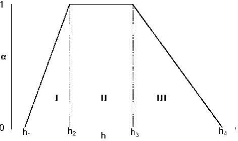
Fig. 1. Root water uptake reduction function, as implemented in

SWAP, after van Dam et al. (2008).

In SWAP, the sink term, S(h), describes the extraction of water by the root architecture at the point macroscopic scale as a function of suction pressure head,h(z,t ). Specif-ically, root water uptake rate at a given soil depth,z, is de-termined by the normalized root density distribution at this depth, β(z,t ), and the maximum transpiration rate, Tmax, whereas reductions due to water stresses are described by the uptake reduction function, α(h)(0≤α≤1), such that

S(h)=β(z,t )·α(h)·Tmax(Kroes and van Dam, 2003). Un-der conditions of no stress, the sink term represents the max-imum uptake rate as follows:Sp=β(z,t )·Tmax.

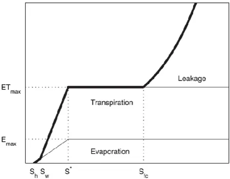
Fig. 2. Loss functionsE(s),T (s), andL(s)as average degree of soil saturation,s, changes in the bucket model due to evaporation, transpiration, and leakage (redrawn from Guswa et al., 2002).

α (h)=       

     

0 , 0≤h < h1

h−h1

h2−h1 , h1≤h < h2 1 , h2≤h≤h3 1− h−h3

h4−h3 , h3< h≤h4 0 , h4< h <+∞

(3)

According to the results by Denmead and Shaw (1962), the value of h3 should depend on potential transpiration and hence, strictly speaking, even the dimensionless parameter

αdepends on the potential transpiration rate. 2.2 The Bucket model

In this work we have used the single-layer bucket model proposed by Laio et al. (2001) and modified by Guswa et al. (2002) that describes soil moisture dynamics at the daily time-scale by assuming the soil as a reservoir to be intermit-tently filled by rainfall events in the form of randomly dis-tributed shots. Soil water storage capacity is emptied by sur-face runoff, deep drainage, and evapotranspiration processes. For this model, the water balance equation at a point scale for the soil layer of depthZr(i.e. the control volume) can be cast as follows:

n Zr

d s (t )

dt =I[s (t ), t]−E[s (t )]−T[s (t )]−L[s (t )] (4)

wheren is soil porosity, and s (0≤s≤1) is the average degree of soil saturation (i.e. the volumetric soil water con-tent,θ, normalized by soil porosity,n)over the entire root-ing zone. In this equation, incomroot-ing (positive) and outgoroot-ing (negative) fluxes are the rate of rainfall infiltrating into the soil, I, the actual evaporation rate,E, the actual transpira-tion rate,T, and the drainage (leakage rate) from the bottom end of the bucket,L, respectively. Note that evaporation,E,

transpiration,T, and leakage,L, rates are considered as func-tion of average soil saturafunc-tion,s, only. Losses due to surface runoff are generated only when the bucket is completely full, i.e. at the condition of full saturation in the soil. Only a frac-tion of the incoming precipitafrac-tion is able to infiltrate into the soil when the rainfall depth exceeds the storage capacity of the soil profile. Therefore, the relationshipI[s(t ),t]=min[r,

nZr(1−s)] accounts for the dependence of infiltration rate,

I, on rainfall depth, r, and the degree of soil saturation,s, in the sense that rainfall infiltration is equal either to rainfall depth or to soil storage capacity, whichever is less. Because of a stochastic representation of precipitation,P (t ), Eq. (4) is a stochastic linear ordinary differential equation and should be viewed as a probabilistic model of soil water budget.

Evapotranspiration is a fundamental hydrologic process and most bucket models treat only implicitly the effect that vegetation canopy exerts on evapotranspiration. An interest-ing feature of the bucketinterest-ing approach proposed by Guswa et al. (2002) is the separation of soil surface evaporation from transpiration by plants. Transpiration,T (s), and evaporation,

E(s), as a function of average soil saturation,s, are computed through the following relations:

T (s)=  



0 , s≤sw

s−sw

s∗_−s

w·Tmax, sw< s < s ∗

Tmax , s≥s∗

(5)

E (s)=  



0 , s≤sh

s−sh

s∗_−s

h ·Emax, sh< s < s ∗

Emax , s≥s∗

(6)

whereswis the saturation at wilting condition, ands∗is sat-uration at incipient stomata closure; the termshis the hygro-scopic saturation, namely the average degree of saturation in soil when soil suction at the soil-atmosphere interface is ex-tremely low (this suction head is often set at a value ranging from 150×103cm to 500×103cm) and evaporation ceases. Depletion of soil water due to the uptake by the plant root system is assumed to be governed by the two major mech-anisms of atmospheric demand and supply of water in the soil. The model does not account for plant characteristics explicitly. Within this framework, a basic soil parameter is the saturation s* when soil water starts becoming a limit-ing factor and plants are no longer able to transpire at the full rate ETmax, as the sum of maximum daily evaporation,

Emax, and maximum daily transpiration,Tmax(see Fig. 2 and Eqs. 5–6). When soil water supply is insufficient to meet the atmospheric demand, namely whensis less thans*, the pro-gressive leaf stomatal closure yields a reduction in root wa-ter uptake and actual transpiration,T, start decreasing from

shaccounts for the fact that evaporation may proceed even after transpiration has stopped at the wilting point of vegeta-tion (Laio et al., 2001). Therefore, fors less thansw, tran-spiration ceases and evaporation from soil surface remains the sole active component of the evapotranspiration process. Other features of the BM can be found in the paper by Guswa et al. (2002).

3 Parameterization strategy for evapotranspiration and field capacity

3.1 Homogenizing BM and SWAP evapotranspiration functions

The bucket and SWAP models handle the calculation of evap-otranspiration rates in different manner and a sort of equiva-lence between them should be set in order to make compar-isons between model outputs meaningful and more effective. A first assumption is that the soil is almost completely cov-ered by vegetative canopies so that soil evaporation can be neglected. From a parametric perspective, this is equivalent to assumesh=swin the BM, while for SWAP soil cover frac-tion,Fsc, is set at 1.0 and crop factor,κc, is also set at 1.0. We basically consider that transpiration water losses follow two stages, the constant and falling rate stages, but do not distinguish between low or high transpiration demands. In SWAP, the falling-rate phase of uptake, and hence of transpi-ration, follows a nonlinear, concave-shaped depletion from

Tmaxto zero (de Jong van Lier et al., 2009). In BM, tran-spiration as a function of average soil saturation in the root zone is modeled by piecewise linear segments as defined by Eq. (5) and shown in Fig. 2. Therefore, to make evapotran-spiration losses of the two models comparable, we impose:

β(z,t )=1 (i.e. uniform root density distribution within the root zone),sw=s(h4)(i.e. equivalence of the wilting points) andh1=h2≈0 (i.e. the effect of the air deficiency negligi-ble). We also sets* such as:

s∗ Z

sw

T (s)·ds+Tmax 1−s∗=Tmax 1 Z

sw

α[h(s)]·ds (7)

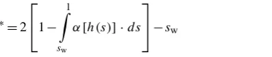
whereT (s)is defined by Eq. (5), whileα(h)is defined by Eq. (3). Equation (7) is equivalent to impose the same av-erage transpiration rate in the soil moisture range from the wilting point to the full saturation condition. Equation (7) is verified ifs* is defined as follows:

s∗=2 

1− 1 Z

sw

α[h(s)]·ds



−sw (8)

Figure 3 shows examples of BM and SWAP transpiration functions after setting parameters* according to Eq. (8).

Fig. 3. BM transpiration function as compared with that of SWAP,

after imposing the condition expressed by Eq. (7).

3.2 Techniques for determining field capacity

Field capacity is defined as the volumetric water content remaining in a uniform soil profile two or three days af-ter having been completely wetted with waaf-ter and afaf-ter free drainage beyond the root zone has become negligible (Soil Sci. Soc. Am., 2008). The field capacity concept was originally introduced for irrigation scheduling purposes un-der a simplistic view of soil water movement in the SVA sys-tem (Veihmeyer and Hendrickson, 1927). It was soon used also by hydrologists who defined it as the maximum quantity of water that can be permanently retained in the soil against the pull of gravity (Horton, 1935). In catchment hydrol-ogy, field capacity is thus considered as a critical threshold parameter of the water-holding capacity of the soil that af-fects both runoff generation mechanism and evapotranspira-tion process. As pointed out by Farmer et al. (2003), the field capacity concept is strictly applicable to the unsaturated zone only and therefore the amount of water held at field capacity will vary as the saturated portion of the soil profile increases or decreases.

suggestedθfc should be related to the hydraulic conductiv-ity function of a soil and determined from theK(θ )-curve as the water content whenK takes on values ranging from 10−6cm s−1 to 10−8cm s−1. Some authors have proposed relating the negligible drainage flux at field capacity,qfc, to the daily evapotranspiration for the area of interest (Kut´ılek and Nielsen, 1994), whereas Laio et al. (2001) defined the field capacity point when drainage losses (Ksin practice, un-der the unit hydraulic gradient assumption) are 10 % of the maximum daily evapotranspiration losses, ETmax.

Whatever the pre-fixed points of theθ (h)orK(θ ) func-tions, soil water content at field capacity is certainly not an inherent soil property, but rather is a process-dependent pa-rameter that may represent only a rough attempt to summa-rize a dynamic flow process through a single global static coefficient (Romano and Santini, 2002). The redistribution process in soil, and hence the field capacity value, depends on the water content distribution established in the entire soil profile at the end of the preceding infiltration phase, as well as on the boundary conditions of the flow domain. In case of coarser-textured soils with stable aggregates, the field capac-ity concept is underpinned by experimental evidence since for these types of soils the drainage process is relatively very fast initially, but then its rates decrease drastically due to the abrupt reduction in unsaturated hydraulic conductivities as suction pressure head increases. Therefore, Romano and Santini (2002) argued that a field drainage experiment is the test to be preferred for determining the water content value at field capacity, namely the condition when drainage fluxes become virtually nil during a redistribution process started from an initially saturated soil profile and with no flux from the soil surface. Using the HYDRUS-1D software to simu-late field drainage experiments for real soils retrieved from different soil databases, Twarakavi et al. (2009) confirmed the inaccuracy of determining field capacity from pre-fixed points of the water retention curve. They also suggested that the value of 0.01 cm day−1can be considered as a negligible drainage flux being imposed at the lower limit of the rooting zone to meet the condition of field capacity for a wide range of soils. Moreover, these authors developed an empirical an-alytical relationship to estimateθfc from information about the soil hydraulic properties.

Especially for practical applications, when judging on the effectiveness of a method with respect to another (for exam-ple, a simplified one) it is important not only to evaluate the discrepancies among parameter values obtained from differ-ent methods (parametric evaluation), but also to analyze the outputs of a hydrologic model computed by using different parameterization techniques (functional evaluation). Under soil, vegetation, and climate conditions representative of a Mediterranean area, a focus here is to compare, with respect to the reference model output, the soil-water budget predic-tions of BM when field capacity is estimated by using either a standard pre-fixed point of theθ (h)curve or a field transient drainage experiment.

Fig. 4. Scatter plots of field capacity,θfc drain, as determined by the

drain-method versus field capacity values obtained from the water

retention characteristics by the fix-method,θfc fix, for the three suc-tion heads of 100 cm, 330 cm, and 500 cm. Data points refer to 1087 soil samples grouped according to different textural classes.

4 Soil, vegetation, and climatic characteristics

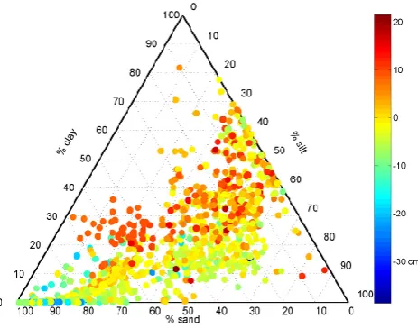
Fig. 5. Ternary diagram of the soil texture triangle showing markers

whose color depends on the magnitude of variable1PAWSmax be-ing the difference between the maximum plant-available soil-water holding capacity when field capacity is alternatively determined us-ing the drain- or fix-method.

gathered from different zones of the World (Nemes et al., 2001) as well as stored in the database of the Soil Hydrology Laboratory of University of Naples Federico II and mainly collected in various parts of Southern Italy (Ceres et al., 2010). On the whole, we have processed data from 1087 soils. Synthetic transient drainage experiments (referred to as drain-method) have been performed to determine the av-erage soil water content, θfc drain, in the soil profile when the drainage rate isqdrain=0.010 cm day−1at the soil depth

zr=1.0 m and imposing a zero flux boundary condition at the soil surface (Romano and Santini, 2002). For the same soils, field capacity (θfc fix)was also calculated from the re-spective water retention functions (referred to as fix-method) as the water content at the fixed suctions heads of 100 cm, 330 cm, and 500 cm (θfc fix−100,θfc fix−330, andθfc fix−500).

Using the entire available dataset and for different soil tex-tural classes, the scatter plots of Fig. 4 provide a qualitative assessment of correlations between variablesθfc drain (hor-izontal axis) and the three different variables θfc fix (verti-cal axes). A 1:1 line is also drawn in each plot to make it easier detecting possible better agreements among the vari-ables. The scatter plots arranged along the principal di-agonal of this kind of matrix diagram (i.e. from the top-left corner to the bottom-right corner of Fig. 4) confirm the higher degree of correlation of θfc drain with θfc fix−100 for coarser soils, withθfc fix−330for medium-textured soils, and with θfc fix−500 for finer soils, respectively (Ceres, 2009). Let PAWSmax=(sfc−sw)×n×Zrbe the maximum plant-available soil-water holding capacity. Then, Fig. 5 illustrates a ternary diagram with relative intensity of each colored dots depending on the magnitude of the difference1PAWSmax= PAWSmax drain−PAWSmax fix when using the sfc drain and

Fig. 6. Boxplots of variable1PAWSmaxfor the soils of the fine, medium, and coarse soil texture classification according to the FAO-HYPRES.

sfc fix values to compute variable PAWSmax. This diagram provides a more quantitative evaluation of the differences among the soils employed in this study and helps in find-ing suitable representative soil samples for the subsequent analyses being carried out in this study. To further proceed in selecting representative soils, we have also grouped all of the 1087 soils according to the classes of the FAO-HYPRES soil textural triangle (Nemes et al., 1999) and computed the boxplots of variable1PAWSmaxfor the soils pertaining to the fine, medium, and coarse textural classes (see Fig. 6). The boxplot for the coarse soil class shows a median approx-imately of−4.3 cm, whereas that one for the fine soil class shows a median approximately of +1.8 cm. With a view to the general aim of this study and based on the results depicted in Figs. 4 to 6, we have considered the soils of the Mediter-ranean area of Southern Italy and selected a loamy-sand soil as representative of coarse soils and a clay soil as representa-tive of fine soils. The major characteristics of these two soil types are presented in the following (see also Table 1).

The physical properties of the loamy-sand soil are as fol-lows: bulk density of 1.198 g cm−3, and USDA percentages of sand, silt, and clay content equal to 73.78 %, 23.27 %, and 2.95 %, respectively. For the clay soil, the physical proper-ties are as follows: bulk density of 1.348 g cm−3, and USDA percentages of sand, silt, and clay content equal to 21.20, 31.80, and 47.00, respectively. For these two differently tex-tured soils, undisturbed soil cores were subjected to evap-oration experiments to obtain the respective parameters of the soil water retention, θ (h), and hydraulic conductivity,

Table 1. Parameters of the van Genuchten-Mualem soil hydraulic relations for the two differently-textured soils used in this study.

Soil texture θr θs αVG nVG K0 τVG

(–) (–) (cm−1) (–) (cm day−1) (–)

Loamy-sand, LS 0.036 0.447 0.025 1.391 86.8 −1.0 Clay, Cl 0.061 0.426 0.0050 1.226 8.81 −1.0

Table 2. BM hydrologic parameters.

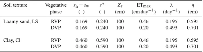
Soil texture Vegetative sh=sw s∗ Zr ETmax λ η phase (–) (–) (cm) (cm day−1) (day−1) (cm)

Loamy-sand, LS RVP 0.169 0.240 100 0.46 0.195 0.595

DVP 0.169 0.240 100 0.20 0.493 0.701

Clay, Cl RVP 0.460 0.590 100 0.46 0.195 0.595

DVP 0.460 0.590 100 0.20 0.493 0.701

Results from the simulation runs are as follows:

sfc drain,LS=0.510 for the loamy-sand soil, andsfc drain,Cl= 0.830 for the clay soil. Instead, adopting the simplified method (referred to as fix-method) of estimating the degree of soil saturation at the field capacity from pre-fixed points of the soil water retention function (see Table 1 for the wa-ter retention paramewa-ters), we obtained the following values:

sfc fix,LS=0.670 for the loamy-sand soil at the suction head of 100 cm, andsfc fix,Cl=0.790 for the clay soil at the suc-tion head of 500 cm. The choice of these two sucsuc-tion heads for computing sfc fix for the coarser soil and the finer soil stems from the results we have presented in Fig. 4.

For both hydrologic models, the control volume is an ac-tive soil profile with a depth of 1.00 m. Therefore, for the bucket model the depth of rooting zone,Zr, is 1.00 m. The porosity values arenLS=0.447 for the loamy-sand soil and

nCl=0.426 for the clay soil. The product nZr represents the so-called active soil depth, which is the volume per unit surface area available for water storage.

For the SWAP model, the lower limit of the root zone is set at a depth of 1.00 m and the entire soil profile was split in three portions accounting for the numerical discretization of the flow domain: the first uppermost portion of 0.10 m in thickness comprises 10 compartments; the second inter-posed portion of 0.40 m in thickness comprises 8 compart-ments, and the third lowermost portion of 0.50 m in thickness comprises 5 compartments. The hydraulic properties of the two different uniform soils are identified by the parameters of Table 1.

Precipitation and transpiration from vegetation are usu-ally out of phase in Mediterranean-type climates being char-acterized by warm and dry summers, during which vege-tation is often under stress conditions, followed by colder

and wet winters where precipitations are predominant and air temperatures are relatively mild. With reference to a hy-drologic year starting on 1 November, we assumed vege-tation dormancy (Dormant Vegevege-tation Phase, DVP) during a wetter rainy period lasting 151 days (from 1 November to 31 March), and the subsequent vegetation regrowth (Re-growth Vegetation Phase, RVP) during a drier and rainless period lasting 214 days (from 1 April to 31 October). During the wetter season, rainfall volume exceeds evapotranspira-tion losses, thus soil “bucket” tends to be filled close to the field capacity. During the drier season, in spring vegetation starts leafing out and exhausting soil water storage by tran-spiration, and when summer is coming transpiration is reg-ulated by the leaf stomatal closures as atmospheric demand increases more and more.

Viola et al. (2008) suggested that in a Mediterranean ecosystem soil moisture dynamics can be effectively in-vestigated by representing the climatic forcing during the year as a sequence of a wet and a dry period, each char-acterized by a stationary rainfall regime. We considered a Mediterranean woodland ecosystem comprising the fol-lowing deciduous species: Quercus pubescens Willd., Acer campestre L., and Fraxinus ornus L. For this woody area, values of maximum evapotranspiration, ETmax, are set con-stant during each season: at 0.46 cm day−1 during the RVP season, and 0.20 cm day−1during the DVP season (Pumo et al., 2008).

To evaluate the impact of the seasonal evolution of rain-fall intensity on soil moisture dynamics, the occurrence of precipitation in time, P (t ), has been probabilistically de-scribed using a Poisson Rectangular Pulse (PRP) model on a daily time scale with probability of occurrence equal to

Table 3. SWAP hydrologic parameters.

Soil texture Vegetative h1=h2 h3 h4=hw Zr ETmax Fsc κc phase (cm) (cm) (cm) (cm) (cm day−1) (–) (–)

Loamy-sand, LS RVP 1.0 300 16 000 100 0.46 1.0 1.0

DVP 1.0 300 16 000 100 0.20 1.0 1.0

Clay, Cl RVP 1.0 1500 16 000 100 0.46 1.0 1.0

DVP 1.0 1500 16 000 100 0.20 1.0 1.0

Table 4. Relative soil moisture at field capacity,sfc, for BM and soil-water storage capacity, WSini, in the system at the start of the simulation run.

Soil texture Method sfc(–) WSini(cm)

Loamy-sand, LS drain (drainage exp.) 0.510 22.80

fix (from Eq. 2a ath=100 cm) 0.670 29.95 Clay, Cl drain (drainage exp.) 0.830 35.36

fix (from Eq. 2a ath=500 cm) 0.790 33.65

(in number of storms per day) does not account for the tem-poral structure within each rainfall event, whereas the distri-bution of storm depth is exponential with a mean depth of

η(in cm per storm). Following Pumo et al. (2008), the se-lected PRP parameter values are: λRVP=0.195 day−1 and

ηRVP=0.595 cm for the RVP period; λDVP=0.493 day−1 andηDVP=0.701 cm for the DVP period.

4.1 Overview of input parameters for BM and SWAP – initial and boundary conditions

To summarize the parameterization strategy employed for the bucket model and the Richards equation based SWAP model discussed in the previous sections, Tables 2, 3, and 4 reports the various parameter values selected for the two different models (Tables 2 and 3, respectively) and for the two dif-ferently textured soils (the loamy-sand soil and the clay soil, respectively).

In view of one specific objective of the present study, Ta-ble 4 reports the values of relative soil moisture at the con-dition of field capacity for the loamy-sand and the clay soils when adopting the drain-method or the fix-method (Romano and Santini, 2002).

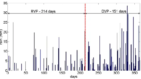
Simulation runs have been carried out using one time-series of synthetic daily rainfall records generated stochasti-cally for a 100-year-long period, obtained by combining two different Poisson Rectangular Pulse (PRP) models, for the regrowth (RVP) and dormant vegetation (DVP) phases, re-spectively. Table 2 reports the PRP parameters for the RVP and DVP periods whereas, as an example, Fig. 7 shows for a generic year the rainfall sequences generated with the PRP model for these two seasons of the hydrologic year.

Fig. 7. Synthetic records of rainfall depth for a generic year. The red

line separates the hydrologic year into the RVP and DVP seasons.

In order for the SWAP lower boundary condition to be ir-relevant or not to affect too much the simulated soil-water balance in the first 1.0 m of rooting depth, the lower end of the flow domain is set at a depth ofzbot=2.0 m from soil surface. The lower boundary condition is specified as the Neumann condition of free drainage, namely the unit gradi-ent of the total hydraulic head [i.e.∇(h−z)= −1] applied at

zbot. Field capacity can be a representative value for the soil water content at the end of the wet season and, for both mod-els, in the first year simulations start when the systems are at the condition of field capacity in soil at the beginning of what we assumed being the growing season (1 April). Therefore, the starting condition is the degree of soil moisturesfc for the bucket model, and the suction headhfc, corresponding to

represents a relatively wet condition for the soil-vegetation system and the relevant values are reported in Table 4 for the two soil types and the two different techniques to determine soil moisture at field capacity. To lessen or remove the ef-fects of the initial conditions on the intercomparison results, the first year of simulation is taken as a sort of spin-up time and removed from the subsequent analyses. Therefore, the actual initial condition is the state of the system at the end of this first year of preliminary simulation. Apart from other forcing variables, a spin-up time for soil moisture varies with the thickness of soil profile: the deeper the soil depth is, the longer the soil moisture reaches its equilibrium state. By run-ning several simulations with different initial conditions, we observed that the results were independent from the initial condition after the first year.

4.2 Performance measures

We have selected the mean error (ME) and the root-mean-square error (RMSE) as performance measures, which are computed using the following equations:

ME=

N

P

i=1 erri

N (9)

RMSE= v u u u t

N

P

i=1

(erri)2

N (10)

whereN is the total number of data and erri =(viSWAP−

v_iBM)represents the deviation between the generic variable,

v_iSWAP, computed by the RE-based SWAP model (assumed as a reference) and the corresponding variable, vBM_i , com-puted by the BM model. The ME statistic reveals the pres-ence of biases (a positive value means that on average the bucket model underestimates) and is a measure of accuracy. The RMSE statistic is a commonly used measure of preci-sion. Both ME and RMSE are dimensional indices and their best values are zero. A feature of RMSE statistic is that it tends to emphasize larger values in a series, whereas lower values are virtually neglected.

5 Results of the numerical experiments and discussion

Using the parameterization strategy outlined in Sect. 3, for the loamy-sand and the clay soils described in Sect. 2.3 we have compared the BM’s hydrologic responses to those of the RE-based SWAP model when in BM the degree of soil saturation at field capacity,sfc, is either determined from a field drainage experiment (drain-method) or estimated as a prefixed point of the soil water retention characteristic (fix-method).

Simulations refer to a well vegetated landscape, and there-fore transpiration is assumed to be dominant to evaporation

within the evapotranspiration processes (i.e.Emax≈0). A preliminary check was carried out to ensure that the gener-ated daily rainfall rate, r, never exceeds the saturated hy-draulic conductivity,Ks, so as to avoid that the occurrence of surface runoff might have led to difficulties when compar-ing the BM and RE-based SWAP performances, and hence to have better similarity among the responses offered by these two hydrologic models.

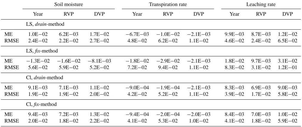
The selected performance indices are reported in Table 5 and show relatively good agreements between the BM and RE outputs, with ME and RMSE absolute values ranging around an order of some percent unit. The worst accuracy (ME = 3.1 %) and precision (RMSE = 12.0 %) for the bucket model occur when field capacity of the loamy-sand soil is determined by the fix-method. Both these largest ME and RMSE values refer to the simulation of leaching rates evolv-ing durevolv-ing the dormant vegetation period and are indica-tion of certain underestimaindica-tions and wider spread of the loss fluxes computed by BM. Based on the ME index, parameter-izingsfc of the loamy-sand soil with the drain-method (see Table 5) leads almost always to the least biased responses. This occurs not only for the entire hydrologic year, but also for both RVP and DVP periods. The type of biases with re-spect to the reference SWAP model depends on the type of variable considered. BM systematically overestimates tran-spiration rate and underestimates leaching rate. In the case of soil moisture the bias behavior is different since there is an underestimation for the drain-method, but an overestima-tion when the fix-method is used. Only for the DVP period of soil moisture variable, the bias in absolute terms is more favorable when the fix-method is used to estimate field ca-pacity. In terms of RMSE (see Table 5), the determination ofsfcwith the drain-method increases the precision of BM responses significantly over the entire hydrologic year: for the loamy-sand soil, there are reductions in RMSE values of about 57.1 % for soil moisture, 33.3 % for transpiration rate, and 44.6 % for draining rate. When splitting the hydrologic year into the two different periods, the reductions in RMSE values are still evident over the RVP period for all of the three variables, but for the DVP period the advantage of the drain-method is much less evident for transpiration rate.

These comparisons among the index values help in under-standing under what circumstances the different methods of parameterization of field capacity can lead to better or poorer performances of the bucket model. With respect to soil tex-ture, overall the water balance in coarser soils feels more the positive effect of determining the field capacity value through a more rigorous method such as the drain-method. When considering seasonality, the dry season of vegetation regrowth (RVP period) appears more sensitive than the wet dormant season (DVP period) to the drain-method of param-eterizing field capacity soil moisture.

Table 5. Performance indices for the loamy-sand (LS) and clay (Cl) soil.

Soil moisture Transpiration rate Leaching rate

Year RVP DVP Year RVP DVP Year RVP DVP

LS, drain-method

ME 1.0E−02 6.2E−03 1.7E−02 −6.7E−03 −1.0E−02 −2.1E−03 9.9E−03 8.7E−03 1.2E−02 RMSE 2.4E−02 2.2E−02 2.7E−02 4.8E−02 6.2E−02 1.1E−02 4.6E−02 2.4E−02 6.5E−02

LS, fix-method

ME −1.3E−02 −1.6E−02 −8.1E−03 −1.8E−02 −2.9E−02 −2.1E−03 1.8E−02 9.7E−03 3.1E−02 RMSE 5.6E−02 5.9E−02 5.2E−02 7.2E−02 9.4E−02 1.1E−02 8.3E−02 3.1E−02 1.2E−01

Cl, drain-method

ME 9.1E−03 7.1E−03 1.1E−02 −9.0E−04 −1.9E−04 −2.1E−03 8.3E−03 6.9E−03 9.0E−03 RMSE 1.9E−02 1.9E−02 2.0E−02 4.2E−02 5.2E−02 1.1E−02 3.9E−02 1.7E−02 5.8E−02

Cl, fix-method

ME 9.4E−03 7.2E−03 1.3E−02 −9.4E−04 −2.0E−04 −2.0E−03 8.4E−03 7.0E−03 1.0E−02 RMSE 2.0E−02 1.8E−02 2.2E−02 4.1E−02 5.3E−02 1.0E−02 4.1E−02 1.8E−02 5.9E−02

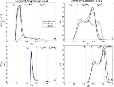
the Fig. 8. For the loamy-sand soil the top plots refer to the RVP (panel a) and DVP (panel b) sub-periods of the hydro-logic year, whereas the bottom plots refer again to the RVP (panel c) and DVP (panel d) sub-periods but for the clay soil. The shapes of thep(s)functions are clearly affected by the climatic forcing imposed during the two different RVP and DVP periods. Comparisons when moving horizontally on Fig. 8 (i.e. from a to b, or from c to d) provide evidence of the occurrence of different seasonal dynamics of the average soil moisture in the active soil profile, with vegetation that modulates interstorm soil moisture redistribution. Note that thep(s)functions of Fig. 5c–d are shifted towards the higher

svalues because of the hydraulic properties of the clay soil, but the general shapes of the PDFs remain nearly unchanged with respect to the effects of both seasonal changes (horizon-tal comparisons) and field capacity parameterization (drain-method vs. fix-(drain-method, i.e. blue solid lines vs. green dotted lines).

Although soil moisture content is obviously bounded be-tween the permanent wilting and porosity points of the spe-cific soil type, the single-peaked p(s)RVP functions of the drier RVP period (Fig. 5a or 5c) have the typical shape of a system characterized by a relatively deep soil profile and low mean rainfall rate (i.e. a low PRP parameterλ). These

p(s)RVPfunctions are positively skewed and narrow distribu-tions, with relative soil moisture contents that vary in a small range around the peak and show quite long tails starting soon after the relative soil moisture points∗ of incipient stomata closure. The modal value located close to the wilting point corresponds to the preferred state over the main part of the RVP, whereas the succeeding long tail located in the right

side of the plot is representative of the fast transition from a wet state at the end of the dormant season toward a nearly dry stationary state. During this vegetative (re-)growing pe-riod, vegetation transpiration dominates the water balance and controls soil moisture contents in the active soil zone, which are consistently low. Consequently, leakage becomes a negligible process. For the fraction of the hydrologic year corresponding to the wetter DVP period (Fig. 5b and 5d), the fluctuation of precipitation and storage capacity of soil are perceived to dominate over the smaller amount of transpira-tion and to exert a remarkable control on soil moisture vari-ability over time. Most of the soil water stored in the system results in unstressed evapotranspiration. The different pre-cipitation regime and transpiration characteristics of this pe-riod basically make thep(s)DVPfunctions to be broader than those of the previous case and more concentrated arounds

values near the field capacity point,sfc.

Fig. 8. Probability density functions of relative soil moisture content,s, for the loamy-sand soil (5a and 5b) and for the clay soil (5c and 5d). The plots on the left-hand-side refer to the RVP season, whereas the plots of the right-hand side refer to the DVP season. Red solid lines are the SWAP model results used as a reference; blue solid lines refer to BM when field capacity is parameterized with the drain-method; green dotted lines refer to BM when field capacity is parameterized with the fix-method.

of the response timescales of soil moisture in the root zone can help in gaining a better understanding of the model com-parisons presented in this study.

The evolution of the dry RVP season depletes soil mois-ture from the rooting zone as precipitation falls only over a small fraction of this period. The depletion time indicates how long it would take the maximum plant-available soil-water holding capacity, PAWSmax=(sfc−sw)×n×Zr, of the soil-vegetation system to dry out subject to the net out-flow,Rd= ETmax−P, between maximum evapotranspiration and mean precipitation rates (P=η·λ), that remains constant and not considering other fluxes (Beljaars et al., 1996; Viola et al., 2008). In a similar way, we can define a replenishment timescale of the soil bucket during the DVP season assuming that the termRr=P−ETmax remains constant throughout that period. Accordingly, the depletion time,td, and the re-plenishment time,tr, give an indication of average moisture residence time in the soil and are calculated as follows:

td=

PAWSmax

Rd

, (11)

tr=

PAWSmax

Rr

. (12)

These two timescales are in Table 6, which also reports the ratiosρdandρrthat relate the depletion and replenish-ment times to the durations of the RVP (214 days) and DVP (151 days) seasons, respectively. The values of ratioρdare fairly similar among them and show that depletion times are approximately 25 % or 20 %, depending on the specific soil type, of the total length of the dry RVP season and this situa-tion, from the one hand, justifies the presence of the extended tails in the soil moisture probability density functions,p(s)

(see Fig. 8a and b). On the other hand, however, it indirectly suggests that the amount of water stored in soil is relatively small for most of this dry period and hence field capacity be-comes a parameter that can exert a more limited influence on the computation of soil water balance.

Table 6. Characteristic time scales of the bucket model during the DVP and RVP periods computed for the loamy-sand (L-S) and the clay

(Cl) soils.

Soil texture Method PAWSmax(cm) RVP (214 days,Rd=0.344 cm d−1) DVP (151 days,Rr=0.146 cm d−1)

td(days) ρd(%) tr(days) ρr(%)

LS draina 15.24 44.3 20.7 104.7 69.3

fixb 22.39 65.1 30.4 153.8 101.9

Cl draina 15.76 45.8 21.4 108.3 71.7

fixc 14.06 40.9 19.1 96.6 63.9

a_{drain =s}

fcdefined by the drainage experiment;bfix =sfcfrom Eq. (2a) ath=100cm;cfix =sfcfrom Eq. (2a) ath=500cm.

the drain-method or the fix-method (and this happens for the loamy-sand soil; see plots 5a and 5b), the worse appear the comparisons between the BM and RE-SWAP models. This discussion provides a more quantitative perspective of our re-sults and also reinforces the significance of the performance indices reported in Table 5. By dwelling on relative soil moisture over the DVP season, we have a reduction in RMSE between the two methods of about 48.1 % for the loamy-sand soil and of about 9.1 % for the clay soil. Instead, for the leaching rates computed over the DVP season there are RMSE reductions of about 45.8 % and 1.7 % for the LS and Cl soils, respectively. As expected, transpiration rates over the DVP season (but over the RVP season, too) as computed by BM are less affected by the techniques used to determine the value of soil moisture at field capacity,sfc.

It is worth noting that thep(s)DVP distributions clearly show a propensity for a temporal bimodality. The DVP bi-modal distribution is characterized by two preferential soil moisture states: a more pronounced peak, to which higher probability is attached, is at around the field capacity value, while another peak is located in proximity tos∗(depending on soil texture). The occurrence of bimodality in the proba-bility distribution of relative soil moisture has been observed and discussed by several researchers (e.g. Kochendorfer and Ram´ırez, 2005; Daly et al., 2009; Vivoni et al., 2010), also with different views. D’Odorico and Porporato (2004) rein-forced previous ideas that a bimodal PDF of soil moisture measurements over the summer season in the continental re-gion of Illinois provided evidence of a soil moisture-rainfall feedback mechanism. Instead, Teuling et al. (2005) argued that an explanation of the soil moisture bimodality observed in Illinois should be the seasonality in meteorological forcing and the nonlinearity of the soil moisture loss function. The data set used by Lee and Hornberger (2006) did not permit to single out any of these hypotheses as the cause for bimodal-ity, and these authors also warned about not making any causality claim since that requires strong statistical support. With specific reference to the stochastic generation of tem-poral precipitation fields, Porporato and D’Odorico (2004) have put forward the hypothesis that Poisson-type noises ap-plied to a nonlinear system can induce, among other things,

a temporal persistence around preferential states and hence a bimodality in the probability density function of relative soil moisture time-series. In this case, the variability of pre-cipitation imposed during the DVP season, and specifically the frequency of storm occurrence, can result in the bimodal shape of thep(s)DVPdistributions depicted in Fig. 8. Over-all, the soil moisture probability distributions in the plots 5b and 5d show that during the DVP period the soil, it being of coarser or finer texture, can preferentially be in either wet states close to field capacity, or relatively drier states closer to the incipient stomata closure. In other words, the bimodality observed in the DVP is representative of two dominant states: one during the transition stage from the dry season to the wet season, when there is a rapid increase of the saturation degree above the stress value threshold; the other corresponding to a stationary wet state.

With respect to the two different methods to determine pa-rametersfc, the soil moisture PDFs of Fig. 8 help in iden-tifying under what circumstances might it be appropriate to use the fix-method to parameterize the bucket model. Com-pared to the SWAP reference model, the performances of the bucket model are acceptable only when one refers to the RVP period (plots 8a and 8c). It is interesting to note that this be-havior occurs independently from the textural properties of the soils considered, but this is also partly due to the narrow shape of the soil moisture probability distributions over the considered regrowing season. In accordance to the perfor-mance indices of Tables 1 and 2 and as one would expect, the larger discrepancies between SWAP and BM during the RVP period occur for the loamy-sand soil and when adopting the fix-method for estimatingsfc. Instead, the plots 5b and 5d pertaining to the dormant and wetter season (DVP period) overall show rather poor performances of the bucket model especially whensfcis estimated by the fix-method and for the coarser soil (Fig. 5b).

Fig. 9. Daily values of the 5th, 50th, and 95th quantiles for the loamy-sand soil over the entire hydrologic year as obtained from the 99 years

of simulation run. Red lines refer to the SWAP model used as a reference, while blue lines refer to BM when field capacity is parameterized either with the drain-method (plots on the left-hand side) or with the fix-method (plots on the right-hand side): (a) and (b) refer to relative soil moisture content,s; (c) and (d) refer to daily transpiration fluxes,T; (e) and (f) refer to daily drainage (leakage) fluxes,L.

one would capture soil moisture dynamics in coarser soils and in the rainiest season of a Mediterranean climatic area.

All the above comments and discussions are also clearly reflected in the representation of Fig. 9 showing the 5th, 50th, and 95th quantiles of relative soil moisture content,s, over the entire hydrologic year as obtained from the 99 years of simulation run. The various plots of this figure pertain to

fix-method. In accordance to the performance indicators of Tables 1 and 2, we observe that the loamy-sand soil of this study is remarkably affected by the method used to deter-mine the field capacity parameter,sfc, and that there is also a change in the magnitude of bias in different parts of the hy-drologic year. Specifically, when the fix-method is employed to estimate sfc, the bucket model systematically underesti-mates the simulated soil moisture during the first nearly 50– 60 days of the year, namely from beginning of April to ap-proximately the end of June, as well as when approaching the period February–March. In practice, when field capacity is parameterized by the fix-method, BM is unable to reproduce the reference storage capacity variations during the periods characterized by highest relative soil moisture values. Bet-ter agreements between the RE-SWAP and BM results are observed for this coarser loamy-sand soil only when relative soil moisture attains its lowest values and reaches the perma-nent wilting point.

One should note that the impacts on relative soil moisture of how to determine the BM parametersfc do not necessar-ily imply similar impacts on water fluxes. Seasonal varia-tions of simulated daily transpiration and drainage (leakage) fluxes outgoing from the system are shown in Fig. 9c–d and 9e–f, respectively, when using either the drain- or fix-method to determine the field capacity parametersfc. Regardless of the method employed to determinesfc (but also regardless the soil types considered, although not shown as said be-fore) the bucket model outputs are not able to capture the temporal evolution of transpiration and leakage losses from the Richards equation based model over both the RVP and DVP seasons. Larger discrepancies between simulated BM and RE-SWAP transpiration fluxes are observed during the RVP season of the hydrologic year, especially at the highest soil moisture contents, and this represents a visual evidence of the performance indices of Table 5 as well as is in accor-dance with the preceding discussion about the role of the field capacity parameter in the computation of the seasonal water balance by a single-layer bucket-type model. At the begin-ning of the RVP season soil tends to be at the condition of field capacity and the discrepancies of BM with respect to RE are soon evident, especially whensfcis estimated through the fix-method (see Fig. 9d during the first 60–70 days of simula-tion). The RVP climate conditions induce a rapid soil mois-ture depletion, as we have discussed before and shown in Table 6, and this decrease insas time increases starts earlier and is somewhat more rapid for the bucket model as its mem-ory capability is small (i.e. its response is fairly rapid to cli-matic forcing) compared to that one offered by the Richards model. This can be viewed as a major reason for the tem-poral lags observed in Fig. 9c and d between the BM and RE-SWAP models over the first stage of the RVP season. Another explanation for the observed time-shift between BM and RE-SWAP transpiration fluxes at the end of the wet sea-son/beginning of dry season can of course be also attributed to the differences in the transpiration functions,T (s), shown

in Fig. 3. In general, the time variations of transpiration fluxes as computed by BM during RVP are in agreement with those from the Richards equation only when soil moistures start attaining lower values and close to the critical moisture values*: the drier are moisture conditions in this soil, the better BM transpiration fluxes follow the time fluctuations of the RE-computed fluxes. Overall, the discussed outcome again reinforces the need and the importance of accounting for local seasonal conditions to evaluate the effectiveness of using one modeling scheme of a soil-vegetation system with respect to another. Comparisons appear to be more satisfac-tory during the DVP period even when the values ofsare rel-atively low. As expected, larger deviations of the BM losses from leakage occur for the loamy-sand soil and during the colder and rainier season straddling over the end of the DVP period and the beginning of the RVP period. The BM model-ing scheme tends to underestimate leakage losses over both the RVP and DVP seasons (see also the positive ME values in Table 5 for this loamy-sand soil), with larger discrepan-cies with respect to RE-SWAP occurring over the DVP sea-son since leakage becomes important under high s-values. It is worth mentioning again that DVP is a relatively wetter season, with greater soil moisture values almost throughout the period and hence more prone to failure in the model in-tercomparison because of the differently estimated values for the field capacity parameter.

6 Conclusions

interest and a novelty, as far as we are concerned, is the possi-bility to further frame this outcome while considering a sea-sonality in the input climatic forcing. At least for the cases considered in this study, the bucket model with field capac-ity as determined by the fix-method provides some relatively good predictions preferably when considering finer textured soils and when soil-water balance refers to a drier season of the hydrologic year and vegetation is in under a regrowing stage (RVP period). It is important to point out, however, that the way with which we have parameterized both BM and SWAP is such so as to make boundary conditions and tran-spiration functions as similar as possible and to perform ef-fective intercomparisons. Finally, analyses of the probability density functions of relative soil moisture content have high-lighted the possible occurrence of bimodality in the shape of curves during the dormant vegetation phase as result of the combination of a dry-to-wet transition and a wetter state in the soil. A discussion on this bimodality is far from the pur-pose of this paper and it can be the subject of a subsequent study.

Appendix A

Abbreviations

BM, bucket model; RE, Richards’ equation; SWAP, Soil Water Atmosphere Plant model; DVP, dormant vegetation phase; RVP, regrowth vegetation phase; ME, mean error; RMSE, root-mean-square error.

Acknowledgements. This work profited from the analyses carried

out by Francesca Ceres during her doctoral period. The authors thank A. J. Guswa for having kindly provided the code and information about the bucket model, as well as for his thorough evaluation and helpful comments. His suggestion of considering characteristic depletion and replenishment times was greatly appreciated. We also thank R. S. Crosbie, L. Peeters and two additional anonymous reviewers for their recommendations and constructive criticisms that have helped to improve this manuscript.

Edited by: H. H. G. Savenije

References

Beljaars, A. C. M., Viterbo, P., Miller, M. J., and Betts, A. K.: The anomalous rainfall over the United States during July 1993: Sen-sitivity to land surface parameterization and soil moisture anoma-lies, Mon. Weather Rev., 124, 362–383, 1996.

Beven, K. J.: Changing ideas in hydrology – The case of physically-based models, J. Hydrol., 105, 157–172, 1989.

Bl¨oschl, G. and Montanari, A.: Climate change impacts - throwing the dice?, Hydrol. Processes, 24, 374–381, 2010.

Braud, I.: Spatial variability of surface properties and estimation of surface fluxes of a savannah, Agric. Forest Meteorol., 89, 15–44, 1998.

Ceres, F.: Parameterizing hydrologic models for the management of agro-forestry systems. Ph.D. dissertation, 187 pp., University of Naples Federico II, available on-line at www.unina.it, 2009 (in Italian).

Ceres, F., Chirico, G. B., and Romano, N.: Functional evaluation of the field capacity concept for water balance analysis under climatic seasonality condition, 2010 General Assembly of EGU, EGU2010-2901, Vienna, 2–7 May 2010.

Clark, M. P., Slater, A. G., Rupp, D. E., Woods, R. A., Vrugt, J. A., Gupta, H. V., Wagener, T., and Hay, L. E.: Framework for understanding structural errors (FUSE): A modular framework to diagnose differences between hydrological models, Water Re-sour. Res., 44, W00B02, doi:10.1029/2007WR006735, 2008. Daly, E., Zinger, Y., Deletic, A., and Fletcher, T. D.:

A possible mechanism for soil moisture bimodality in humid-land environments, Geophys. Res. Lett., 36, L07402, doi:10.1029/2008GL036933, 2009.

de Jong van Lier, Q., Dourado Neto, D., and Metselaar, K.: Modeling of transpiration reduction in van Genuchten-Mualem type soils, Water Resour. Res., 45, W02422, doi:10.1029/2008WR006938, 2009.

Denmead, O. T. and Shaw, R. H.: Availability of soil water to plants as affected by soil moisture content and meteorological condi-tions, Agron. J., 54, 385–390, 1962.

D’Odorico, P. and Porporato, A.: Preferential states in soil moisture and climate dynamics, Proc. Natnl. Acad. Sci., 101, 8848–8851, 2004.

Farmer, D., Sivapalan, M., and Jothityangkoon, C.: Climate, soil, and vegetation controls upon the variability of water bal-ance in temperate and semiarid landscapes: Downward ap-proach to water balance analysis, Water Resour. Res., 39, 1035, doi:10.1029/2001WR000328, 2003.

Feddes, R. A., Hoff, H., Bruen, M., Dawson, T., de Rosnay, P., Dirmeyer, P., Jackson, R. B., Kabat, P., Kleidon, A., Lilly, A., and Pitman, A. J.: Modeling root water uptake in hydrological and climate models, B. Am. Meteorol. Soc., 82, 2797–2809, 2001. Guswa, A. J., Celia, M. A., and Rodriguez-Iturbe, I.: Models of soil

moisture dynamics in ecohydrology: A comparative study, Water Resour. Res., 38, W01166, doi:10.1029/2001WR000826, 2002. Holl¨ander, H. M., Blume, T., Bormann, H., Buytaert, W., Chirico,

G. B., Exbrayat, J.-F., Gustafsson, D., H¨olzel, H., Kraft, P., Stamm, C., Stoll, S., Bl¨oschl, G., and Fl¨uhler, H.: Comparative predictions of discharge from an artificial catchment (Chicken Creek) using sparse data, Hydrol. Earth Syst. Sci., 13, 2069– 2094, doi:10.5194/hess-13-2069-2009, 2009.

Horton, R. E.: Surface runoff phenomena: I. Analysis of the hydro-graph, Horton Hydrol. Lab. Pub. 101, Vorheesville, N.Y., 73 pp., 1935.

Kochendorfer, J. P. and Ram´ırez, J. A.: The impact of land atmo-sphere interactions in the temporal variability of soil moisture, J. Hydrometeorology, 6, 53–67, 2005.

Kowalczyk, E. A., Wang, Y. P., Law, R. M., Davies, H. L., Mc-Gregor J. L., and Abramowitz, G.: The CSIRO Atmosphere Bio-sphere Land Exchange (CABLE) model for use in climate mod-els and as an offline model, CSIRO Marine and Atmospheric Re-search, Paper #13, 257 pp., 2006.

Kut´ılek, M. and Nielsen, D. R.: Soil Hydrology. GeoEcology Text-book, Catena Verlag, Cremlingen-Destedt, Germany, 1994. Laio, F., Porporato, A., Ridolfi, L., and Rodriguez-Iturbe, I.: Plants

in water controlled ecosystems: Active role in hydrological pro-cesses and response to water stress, II. Probabilistic soil moisture dynamics, Adv. Water Resour., 24, 707–723, 2001.

Lee, D. H. and Abriola, L.: Use of the Richards equation in land surface parameterizations, J. Geophysical Res., 104, 519–526, 1999.

Lee, T. R. and Hornberger, G. M.: Inferred bimodality in the distribution of soil moisture at Big Meadows, Shenandoah National Park, Virginia, Geophys. Res. Lett., 33, L06407, doi:10.1029/2005GL025536, 2006.

Manabe, S.: The atmospheric circulation and the hydrology of the earth’s surface, Mon. Weather Rev., 97, 739–774, 1969. Manus, C., Anquetin, S., Braud, I., Vandervaere, P., Creutin,

J.-D., Viallet, P., and Gaume, E.: A modeling approach to assess the hydrological response of small mediterranean catchments to the variability of soil characteristics in a context of extreme events, Hydrol. Earth Syst. Sci., 13, 79–97, doi:10.5194/hess-13-79-2009, 2009.

Meyer, P. D. and Gee, G. W.: Flux-based estimation of field capac-ity, J. Geotechnical Geoenvironmental Engineering, 125, 595– 599, 1999.

McDonnell, J. J., Sivapalan, M., Vach´e, K., Dunn, S., Grant, G., Haggerty, R., Hinz, C., Hooper, R., Kirchner, J., Roderick, M. L., Selker, J., and Weiler, M.: Moving beyond heterogeneity and process complexity: A new vision for watershed hydrology, Water Resour. Res., 43, W07301, doi:10.1029/2006WR005467, 2007.

Milly, P. C. D.: Climate, soil water storage, and the average annual water balance, Water Resour. Res., 30, 2143–2156, 1994. Milly, P. C. D., Betancourt, J., Falkenmark, M., Hirsch, R. M.,

Kundzewicz, Z. W., Lettenmaier, D. P., and Stouffer, R. J.: Sta-tionarity is dead: Whither water management?, Science, 319, 573–574, 2008.

Nemes, A., W¨osten, J. H. M., Lilly, A., and Oude Voshaar, J. H.: Evaluation of different procedures to interpolate particle-size dis-tributions to achieve compatibility within soil databases, Geo-derma, 90, 187–202, 1999.

Nemes, A., Schaap, M. G., Leij, F. J., and W¨osten, J. H. M.: De-scription of the unsaturated soil hydraulic database UNSODA version 2.0, J. Hydrol., 251, 151–162, 2001.

Oleson, K. W., Lawrence, D. M., Bonan, G. B., Flanner, M. G., Kluzek, E., Lawrence, P. J., Levis, S., Swenson, S. C., and Thorn-ton, P. E.: Technical Description of version 4.0 of the Commu-nity Land Model (CLM), NCAR Technical Note, NCAR/TN-478+STR, Boulder, CO, 2010.

Porporato, A. and D’Odorico, P.: Phase transitions driven by state-dependent Poisson noise, Phys. Rev. Lett., 92, 110601, doi:10.1103/PhysRevLett.92.110601, 2004.

Porporato, A., D’Odorico, P., Laio, F., Ridolfi, L., and Rodriguez-Iturbe, I.: Ecohydrology of water-controlled ecosystems, Adv. Water Resour., 25, 1335–1348, 2002.

Pumo, D., Viola, F., and Noto, L. V.: Ecohydrology in Mediter-ranean areas: a numerical model to describe growing seasons out of phase with precipitations, Hydrol. Earth Syst. Sci., 12, 303– 316, doi:10.5194/hess-12-303-2008, 2008.

Romano, N. and Santini, A.: Determining soil hydraulic func-tions from evaporation experiments by a parameter estimation approach: Experimental verifications and numerical studies, Wa-ter Resour. Res., 35, 3343–3359, 1999.

Romano, N. and Santini, A.: Water retention and storage: Field, in: Methods of Soil Analysis, Part 4, Physical Methods, edited by: Dane, J. H. and Topp, G. C., 721–738, SSSA Book Series N.5, Madison, WI, USA, 2002.

Romano, N., Brunone, B., and Santini, A.: Numerical analysis of one-dimensional unsaturated flow in layered soils, Adv. Water Resour., 21, 315–324, 1998.

Seneviratne, S. I., Corti, T., Davin, E. L., Hirschi, M., Jaeger, E. B., Lehner, I., Orlowsky, B., and Teuling, A. J.: Investigating soil moisture – climate interactions in a changing climate: A review, Earth-Sci. Rev., 99, 125–161, 2010.

Settin, T., Botter, G., Rodriguez-Iturbe, I., and Rinaldo, A.: Numerical studies on soil moisture distributions in het-erogeneous catchments, Water Resour. Res., 43, W05425, doi:10.1029/2006WR005737, 2007.

Sharma, M. L. and Luxmoore, R. J.: Soil spatial variability and its consequences on simulated water balance, Water Resour. Res., 15, 1567–1573, 1979.

ˇSim˚unek, J., ˇSejna,, M., Saito, H., Sakai, M., and van Genuchten, M. T.: The Hydrus-1D Software Package for Simulating the Movement of Water, Heat, and Multiple Solutes in Variably Sat-urated Media, Version 4.0, HYDRUS Software Series 3, Depart-ment of EnvironDepart-mental Sciences, University of California River-side, RiverRiver-side, California, USA, 315 pp., 2008.

Soil Science Society of America: Glossary of soil science terms. SSSA, 92 pp., Madison, WI, ISBN 978-0-89118-851-3, 2008. Sposito, G.: The “physics” of soil water physics, Water Resour.

Res., 22, 83S–88S, 1986.

Teuling, A. J., Uijlenhoet, R., and Troch, P. A.: On bimodality in warm season soil moisture observations, Geophys. Res. Lett., 32, L05404, doi:10.1029/2005GL023223, 2005.

Twarakavi, N. K. C., Sakai, M., and ˇSim˚unek, J.: An objective anal-ysis of the dynamic nature of field capacity, Water Resour. Res., 45, W10410, doi:10.1029/2009WR007944, 2009.

van Dam, J. C., Groenendijk, P., Hendriks, R. F. A., and Kroes, J. G.: Advances of modeling water flow in variably saturated soils with SWAP, Vadose Zone J., 7, 640–653, 2008.

Veihmeyer, F. J. and Hendrickson, A. H.: Soil moisture conditions in relation to plant growth, Plant Physiol., 2, 71–78, 1927. Viola, F., Daly, E., Vico, G., Cannarozzo, M., and Porporato,

A.: Transient soil-moisture dynamics and climate change in Mediterranean ecosystems, Water Resour. Res., 44, W11412, doi:10.1029/2007WR006371, 2008.