Nitrogen surface water retention in the Baltic Sea drainage basin

www.hydrol-earth-syst-sci.net/19/981/2015/ doi:10.5194/hess-19-981-2015

© Author(s) 2015. CC Attribution 3.0 License.

Nitrogen surface water retention in the Baltic Sea drainage basin

P. Stålnacke1, A. Pengerud1, A. Vassiljev2, E. Smedberg3, C.-M. Mörth3, H. E. Hägg3, C. Humborg3, and H. E. Andersen4

1_{Bioforsk – Norwegian Institute for Agricultural and Environmental Research, Fr. A. Dahls vei 20, 1430 Ås, Norway} 2_{Tallinn University of Technology, Ehitajate tee 5, Tallinn 19086, Estonia}

3_{Baltic Sea Centre, Stockholm University, 106 91 Stockholm, Sweden}

4_{Aarhus University, Department of Bioscience, Vejlsøvej 25, 8600 Aarhus, Denmark}

Correspondence to: P. Stålnacke (per.stalnacke@bioforsk.no)

Received: 15 August 2014 – Published in Hydrol. Earth Syst. Sci. Discuss.: 26 September 2014 Revised: – – Accepted: 20 January 2015 – Published: 23 February 2015

Abstract. In this paper, we estimate the surface water re-tention of nitrogen (N) in all the 117 drainage basins to the Baltic Sea with the use of a statistical model (MESAW) for source apportionment of riverine loads of pollutants. Our re-sults show that the MESAW model was able to estimate the N load at the river mouth of 88 Baltic Sea rivers, for which we had observed data, with a sufficient degree of precision and accuracy. The estimated retention parameters were also sta-tistically significant. Our results show that around 380 000 t of N are annually retained in surface waters draining to the Baltic Sea. The total annual riverine load from the 117 basins to the Baltic Sea was estimated at 570 000 t of N, giving a total surface water N retention of around 40 %. In terms of absolute retention values, three major river basins account for 50 % of the total retention in the 117 basins; i.e. around 104 000 t of N are retained in Neva, 55 000 t in Vistula and 32 000 t in Oder. The largest retention was found in river basins with a high percentage of lakes as indicated by a strong relationship between N retention (%) and share of lake area in the river drainage areas. For example in Göta älv, we estimated a total N retention of 72 %, whereof 67 % of the retention occurred in the lakes of that drainage area (Lake Vänern primarily). The obtained results will hopefully en-able the Helsinki Commission (HELCOM) to refine the nu-trient load targets in the Baltic Sea Action Plan (BSAP), as well as to better identify cost-efficient measures to reduce nutrient loadings to the Baltic Sea.

1 Introduction

Expanding human activities have had a great impact on nutri-ent dynamics and nutrinutri-ent export from watersheds (Hill and Bolgrien, 2011; Mayorga et al., 2010). Increased population densities, food production, sewage emissions and fossil fuel combustion are among the driving forces causing increased nutrient mobilisation and alterations to hydrological systems (Mayorga et al., 2010). Increased nutrient export from coastal watersheds has had severe impacts on the ecological func-tions and community composition of estuaries, with algal blooms, increased water turbidity, oxygen depletion, and se-vere fish deaths as the most prominent consequences (Kel-logg et al., 2010; Mayorga et al., 2010; Hoffmann et al., 2009).

watersheds could retain as much as 60–90 % of total N inputs (Kellogg et al., 2010). Reduced N export can be achieved by increasing N retention in soils, sediments and biomass, re-ducing atmospheric and terrestrial N sources, and increasing in-stream N removal and retention processes (Hill and Bol-grien, 2011).

Water residence time is a major factor determining the re-tention of nutrients in watersheds (Hejzlar et al., 2009), while Hesse and co-workers emphasised the need for better un-derstanding of terrestrial retention (i.e. in soils; Hesse et al., 2013). Watershed characteristics, such as hydrology and ge-omorphology, strongly control water residence time, and in-creased water residence time can enhance denitrification pro-cesses and thereby reduce N loads to coastal waters (Kellogg et al., 2010; Behrendt and Opitz, 2000). Total N inputs in-fluence denitrification rates, whereas hydrology and geomor-phology (or water residence time) influence the proportion of N inputs that are denitrified (Seitzinger et al., 2006). Cer-tain areas within watersheds can be identified as sink areas with regard to N export, often being areas with a relatively long water residence time where biogeochemical processes can transform reactive N into organic N in biomass, or N gases via denitrification (Kellogg et al., 2009), or burial of N in sediments (Harrison et al., 2009). The mitigating effect of these sink areas could in some cases be negligible, especially in cases where such areas are bypassed by N-carrying wa-ter flows due to specific land management practices (e.g. tile drains or storm water overflows) (Kellogg et al., 2009). Den-itrification processes are favoured in sediments and hypoxic or anoxic bottom waters, particularly in systems with abun-dant organic carbon (C) and nitrate (Harrison et al., 2009; Mulholland et al., 2008).

The question on how to quantify the retention of nutrients from source to river mouth remains one of the largest un-certainties in river basin management. Several authors (e.g. Mayorga et al., 2010; Seitzinger, 2008) emphasise the need for advances in methods and models for determining the im-pacts of human activities on nutrient inputs to coastal wa-ters, and a better understanding of the processes leading to retention of N in watersheds. Seitzinger et al. (2002) argue that studies generally have focused on N removal in shorter sub-sections of rivers and emphasise the need for a river net-work approach if we are to quantify the retention of nutrients relative to total inputs. In later years, a number of models of different complexity have been developed for estimating surface water N retention (e.g. Billen et al., 2009; Grimvall and Stålnacke, 1996; Hejzlar et al., 2009; Hill and Bolgrien, 2011; Jung and Deng, 2011; Mayorga et al., 2010; Seitzinger et al., 2002).

In this paper, we estimate the surface water retention of N in the Baltic Sea drainage basin with the use of a statistical model for source apportionment of riverine loads of pollu-tants, the MESAW model (Grimvall and Stålnacke, 1996). Scientifically, estimation of retention is one of the largest challenges in river basin nutrient accounting (i.e. source

ap-portionment and budget calculations) and, therefore, also the case in the Baltic Sea drainage basin.

2 Materials and methods

The Baltic Sea, together with the lakes and watercourses in its drainage basin, represents one of the most intensively monitored aquatic systems in the world and eutrophication has been identified as a major threat to this system. The total area of the Baltic Sea drainage basin is 1 745 000 km2, which is around four times the area of the sea itself. The long-term average inflow of freshwater with the rivers is 475 km3yr−1 or 15 130 m3s−1 (Bergström and Carlsson, 1994; Mörth et al., 2007). Details on population and land use characteris-tics in the Baltic Sea drainage area can be found in Mörth et al. (2007).

2.1 MESAW input data Model input data included

1. land cover, including cultivated land, wetland, lake area, other land (mainly forest), and total drainage area (Corine Land Cover 2006 raster data);

2. atmospheric N wet deposition (EMEP; http://emep.int/ publ/helcom/2012/index.html);

3. point source emissions, including emissions from waste water treatment plants (WWTPs) and industry (data from HYDE, EUROSTAT and OECD);

4. observed annual riverine N load (kg N yr−1) as esti-mated from riverine N concentration and water dis-charge data for the time period 1994–2006 (PLC database by HELCOM (www.helcom.fi) and data from Denmark from NERI).

Based on these national statistics, the total number of “con-nected” people in each country was calculated. The num-ber of “connected” people was then spatially distributed to the grid cells. The distribution was made based on the as-sumption that urban populations and grid cells with higher population numbers would be more likely to have a munic-ipal WWTP connection than rural and smaller populations. Applying this principle, the grid cells for each country were classified as “connected” starting with urban populations in a descending order, and continuing with rural population in the same way until the number of “connected” people reached the number specified by the national statistics. This proce-dure was carried out for all three treatment types; first ter-tiary, then secondary and last primary. The number of people “not connected” to any type of treatment plant was also cal-culated for each grid cell. Total N emission from WWTPs was then calculated for each grid cell based on the approach of Mörth et al. (2007).

2.2 The MESAW model and model parameterisation MESAW is a statistical model for source apportionment of riverine loads of pollutants developed by Grimvall and Stål-nacke (1996). This model approach uses non-linear regres-sion for simultaneous estimation of export coefficients to sur-face waters for the different specified land cover or soil cate-gories and retention coefficients for pollutants in river basins. Examples of application of the MESAW model are given in Lidèn et al. (1999), Vassiljev and Stålnacke (2005), Vassiljev et al. (2008) and Povilaitis et al. (2012). MESAW has many features in common with the more well-known SPARROW model developed in the USA (Smith et al., 1997; Alexander et al., 2000).

The basic principles and major steps in the procedure in-cluded (i) estimation of mean annual riverine N loads for a fixed time period (i.e. the years 1994–2006) at each of the 88 monitoring sites; (ii) derivation of statistics on land cover, lake area, point source emissions and atmospheric deposition (see Sect. 2.1) for each river basin; and (iii) use of a general non-linear regression expression with N loads at each river basin as the dependent/response variable and basin character-istics as covariates/explanatory variables. This gave the fol-lowing generalised form of the model (Eq. 1):

Li= n

X

i=1

(1−R)Si+(1−R)Pi+(1−R)Di+εi, (1)

i=1,2, . . ., n,

where Li is the load at outlet of basin i; Si is total losses from soil to water in basini;Piis the point source discharges (WWTP and industry) to waters in basini;Di is the atmo-spheric deposition on surface waters in sub-basin i; R de-notes the retention for the source emissionsS, P andD, re-spectively;nis the number of basins, andεi is the statistical error term.

The parameterisation of the model is flexible and study-area specific depending on the data and expert knowledge. The model is fitted by minimising the sum of squares for the differences between observed and estimated loads. The model can be run based on absolute or relative values. If based on absolute values, the optimisation procedure finds the minimum sum of squares of the absolute differences be-tween observed and estimated transport. This procedure im-plies that the influence of the different rivers/basins will be a function of size. If relative values are used, the optimisa-tion procedure finds the minimum sum of squares of relative differences between observed and estimated transport. This procedure assumes that all rivers have the same weight in the optimisation routine. In this study, we used relative values in order to give equal weight to small and large river basins.

The total diffuse loss of N from soil to water,Si, in the ith sub-basin was assumed to be a function of the land cover (Eq. 2):

Si=(θ1a1i+θ2a2i+θ3a3i), (2a) wherea1i, a2i anda3iin our study refer to the areas of three land cover classes, i.e. cultivated land, wetlands and other land (mainly forests), respectively.θ1, θ2andθ3are unknown emission coefficients for the three land use categories that are statistically estimated in MESAW jointly with the retention (see Eq. 3 below). The point source emissions,Pi,and atmo-spheric deposition on surface waters,Di, were assumed to be known (see Sect. 2.1).

Throughout the exploratory analysis we found that certain basins deviated from the relationship and in most cases also where geographically located near to each other. Thus, we introduced a “grouping variable” according to the following: Si=(θ1a1i+θ2a2i+θ3a3i)·ωj, (2b) where each groupj consisted of 2 or more basins depend-ing on the model run (see Table 1) and whereωis the un-known coefficient(s). The model was run with different com-binations of basin sub-groups in order to obtain reasonable model coefficients and load estimates (i.e. little deviation be-tween predicted and observed loads). The grouping of basins was based on prior knowledge of similarities between basins as well as geographic location. For example, the 10 smaller Danish sub-basins formed one group, as a residual analy-sis showed that these sub-basins deviated from the general relationships. In its practical meaning, we simply adjusted the “global” diffuse emission coefficients to the local condi-tions (despite not knowing the underlying causes). This can be justified since applying the same coefficient to such a large drainage basin (1 745 000 km2) seem less logic.

Table 1a. Results from the different MESAW model runs for estimation of total nitrogen (N) retention with different combinations of basin sub-groups. Results include estimated export coefficients (kg km−2) from different land use classes (i.e. cultivated, wetland and other), estimated retention coefficients (dimension-less) for lake area and total drainage area, and the coefficient of determination (R2) between observed and predicted annual loads. Standard error (SE) andtratio of the estimated coefficients are given for each model run.

Diffuse emissions Retention

Cultivatedθ1 Wetlandθ2 Otherθ3 Lake In-stream

Model run (kg km−2) (kg km−2) (kg km−2) λ2a λ1a R2b

1 88 monitored basins (1 group) Est. coeff. 1435 405 233 9 4×10−3 0.94

SE 929 2527 443 16 4×10−3

tratio 1.54 0.16 0.53 0.57 1.03

2 88 monitored basins (3 groups) Est. coeff. 1440 386 185 8 2×10−3 0.98

SE 172 753 136 5 5×10−4

tratio 8.38 0.51 1.36 1.78 3.60

3 88 monitored basins (4 groups) Est. coeff. 1137 208 220 11 8×10−4 0.99

SE 115 668 126 5 3×10−4

tratio 9.88 0.31 1.75 2.16 2.62

4 88 monitored basins (5 groups) Est. coeff. 1073 158 225 12 7×10−4 0.99

SE 109 675 123 5 3×10−4

tratio 9.85 0.23 1.83 2.23 2.27

a_{dimensionless;}b_{observed vs. predicted.}

retention mechanism, the parameterisation of the retention in the different basins was after several exploratory runs with alternative models done with the following empirical func-tion (Eq. 3):

Ri=1−

1

1+λ1pdrainage area_i

· 1

1+λ2_{drainage area}lake areai

i

, (3)

i=1,2, . . ., n,

whereλ1andλ2denote a non-negative parameter andRi de-notes the retention in theith basin. The empirical function were in our case derived from the conception that the re-moval of N takes place primarily in the surface waters (both in-streams and in lakes). The first part of the function reflects the in-stream retention whereas the second part reflects the retention in lakes and reservoirs. Our assumption was that the removal rate is proportional to drainage basin size and the ratio of the lake to the total drainage area. Subsequently this can be seen as an indirect expression of the water resi-dence time in the river basin.

Moreover, for the sake of simplicity, we assumed that the retention is the same for source categories D, S and P. Finally, by combining the parametric expressions of losses from soil to waters and retention with the empirical data, the θ1, θ2,θ3,λ1, λ2andωparameters were estimated simultane-ously.

Table 1b. Estimated group ratios±standard error for diffuse emis-sions coefficients.

Model Ratio±SE

run Basin sub-group ωj

2 2 Pregolia, Narva 0.3±0.2

3 Daugava, Neva 2.2±0.3

3 2 Pregolia, Narva 0.4±0.2

3 Daugava, Neva 2.0±0.3 4 10 Danish+6 Swedish 2.0±0.8 (south-west coast) basins

4 2 Pregolia, Narva 0.4±0.2

3 Daugava, Neva 2.0±0.2 4 10 Danish+6 Swedish 2.1±0.8 (south-west coast) basins

5 27 Finnish basins 1.1±0.2

3 Results and discussion 3.1 Parameterisation results

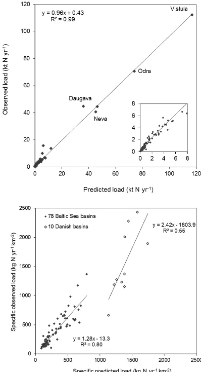
Figure 1. Relationship between observed and predicted annual N load (kt N yr−1; upper panel) and specific observed and predicted N load (kg N yr−1km−2; lower panel) in the 88 Baltic Sea basins with observed N load (lower panel).

(no. 4 in Table 1 with nine estimated parameters), including all 88 basins with observed N load, both retention parame-ters (λ1andλ2) and land use category “cultivated” (i.e.θ1) were statistically significant (p <0.05). The land use cate-gory “other” (θ2which basically is the forest land) was very close to being statistically significant (p <0.06). “Wetland” (θ3) was not statistically significant, but this land use cate-gory accounts for less than 4 % of the total drainage area in the Baltic Sea drainage basin. It should be noted that the clas-sification of wetlands is rather rough from the data source and given as joint expression of all wetlands ranging from marshes to peatland bogs. All four grouping parametersω1– ω4were statistically significant.

It is worth noting that these diffuse losses parameters (θ1−θ3) all are given in kilograms per square kilometres and thus can be interpreted as export or unit-area loss coeffi-cients. Interestingly, our estimates corroborate well with the

Figure 2. Total estimated nitrogen (N) load (kt N yr−1) in the 117 basins of the Baltic Sea drainage area. Total retention is given as the difference between the estimated total load if no retention and the estimated total riverine net N load.

results of monitored losses from small catchments with rel-ative uniform land use. For example, the point estimate and standard error for cultivated land gave an estimate of 1073 and 109 kg km−2, respectively (model run no. 4; Table 1). Stålnacke and co-workers compiled data from 35 small agri-cultural catchments in the Nordic and Baltic regions (Stål-nacke et al., 2014). They found that a majority of these catch-ments had a unit-area loss of between 600 and 2500 kg km−2. In addition, our results showed that the nitrogen losses from agricultural land were almost four times higher than the cor-responding losses from forested land (Table 1), which is found to be realistic and in line with other results (Lidèn et al., 1999; Vassiljev and Stålnacke, 2005; Vassiljev et al., 2008)

3.2 Major retention estimate results

The final model parameterisation using the 88 river basin data (i.e. model run no. 4 in Table 1) was used to determine the surface water retention of N in all 117 major river basins in the Baltic Sea drainage area. This included 78 river basins with observed N load (excluding the 10 smaller Danish sub-basins), and also an additional 39 unmonitored river basins.

Figure 3. Relative total nitrogen (N) retention in the Baltic Sea drainage basins.

around 104 000 t of N are retained in Neva, 55 000 t in Vistula and 32 000 t in Oder (Table A2).

Most of the retention occurs in lakes, as indicated by a strong relationship between N retention (%) and share of lake area in the river drainage areas (up to 20 % lake area; Fig. 4). In Göta älv, we estimated a total N retention of 72 %, whereof 67 % occurred in the lakes of that drainage area (Lake Vänern primarily). Other river basins with high retention were Kymi-joki (70 %), Motalaström (73 %) and Neva (74 %). All these basins are characterised by a high percentage of lakes. Low retention was estimated for lake-poor basins, e.g. Aurajoki (2 %), Kasari (4 %) and Kelia (3 %). This is in accordance with earlier studies, where the highest N retention has been found in river basins with a large proportion of lakes. In a comparison of N retention in four selected watersheds in Eu-rope, representing a wide range in climate, hydrology and nu-trient loads, Hejzlar et al. (2009) found the highest retention values in the two watersheds with lakes as compared to the two other mostly or entirely lake-less watersheds. A global-scale analysis by Harrison et al. (2009) indicated that lakes and reservoirs are important sinks for N in watersheds, with small lakes (<50 km2) retaining about half of the global to-tal. Despite the fact that reservoirs occupy only 6 % of global lentic surface area, the reservoirs were estimated to retain about 33 % of the total N retained by lentic systems.

Figure 4. Relationship between estimated retention (%) and total drainage area (km2; upper panel) and share of lake area (% of total drainage area; lower panel) for 117 Baltic Sea basins.

3.3 Uncertainty aspects and outlook

Figure 5. Relationship between specific N load (kg N km−2) and share of (a) cultivated, (b) wetland, (c) lake and (d) other areas (in % of total drainage area) in the 88 (78 for wetland) Baltic Sea basins with observed N load.

modelling efforts that combine comprehensive data sets on population, land cover, water discharge and quality, etc., may serve as important tools for improved watershed manage-ment and for better identification of cost-efficient measures to reduce nutrient loading. In our study, the MESAW model was apparently able to estimate the N load at the river mouth of 88 Baltic Sea rivers for which we had observed data with a sufficient degree of accuracy (Fig. 1, upper panel; Table 1). However, when we show the obtained relationships using unit-area (specific) load, the model underestimates the load (Fig. 1, lower panel). It is also worth noting that the 10 Dan-ish sub-basins included (despite the effort with the grouping) deviate from the general relationship. These 10 smaller sub-basins have a high observed specific N load, which is not well predicted by the model.

Figure 5a–d show the relationships between observed spe-cific N load (kg N km−2)and share of various land cover cat-egories and lake area in the 88 (78 for wetland) Baltic Sea basins with observed N loads. A high specific N load was generally found in river basins with a large share of culti-vated land, as indicated by a strong positive relationship be-tween specific N load (kg N km−2) and share of cultivated land (%; Fig. 5a). In contrast to cultivated land, the specific N load was found to be negatively correlated with the share of “other land” (i.e. primarily forest; Fig. 5d).

In their modelling of riverine N transport to the Baltic Sea, Mörth et al. (2007) found diffuse sources contribute the most to the overall simulated riverine N loads. A review by

Stål-nacke et al. (2009) also emphasized the importance of dif-fuse sources (or share of cultivated land) in contributing to N loads in watersheds. HELCOM (2011) reports that 45– 61 % of the total waterborne inputs of N to the Baltic Sea are from diffuse sources. The importance of wetlands in deter-mining N loads seems highly variable, with no apparent re-lationship between specific N load and share of wetland area in the river basins (Fig. 5b). This was less surprising since this land cover class included all kinds of wetlands (from marshes to peatlands). The low specific load for drainages in basins with a wetland coverage exceeding 15 % are all lo-cated in middle/northern Finland and also in the northern part of Sweden (Table A1). These basins are all characterised by low population density and low share of cultivated land. In a meta-analysis of the importance of wetlands for the removal of inorganic N and reduction of N export from watersheds, Jordan et al. (2011) found a large variation (0.25–100 %) in N removal efficiency between individual wetlands. When grouped into different wetland classes, mean efficiency was highest for palustrine forested wetlands (63 %) and lowest for estuarine emergent wetlands (33 %).

Regarding statistical uncertainty in our study, the three land cover classes (and the surface water area) add up to 100 % and apparently these explanatory variables are inter-correlated. This will have less influence on the method ap-plied although there is always a risk of multicollinearity in these kinds of regression-type of models. It should be noted that the model inputs are areas of the land cover and not the percentages which will decrease the risk of multicollinear-ity. Experiences with the MESAW models, as also given in the previously quoted papers, in different geographical areas (Lidèn et al., 1999; Vassiljev and Stålnacke, 2005; Vassiljev et al., 2008; Povilaitis et al., 2012) have not indicated any problem with possible interrelated explanatory variables. In addition, the parameter estimates showed reasonable stabil-ity; little change occurred in the values of the most statisti-cally significant model coefficients when additional variables were added in exploratory regressions (Table 1).

The predicted climate change is an additional factor that may significantly affect nutrient loads and retention in wa-tersheds (Jeppesen et al., 2011). Changes in temperature and precipitation will most likely induce changes in agricultural land use, e.g. type of crops grown, rates and timing of fer-tiliser use, and thereby influence N cycling and export to coastal waters. However, given the uncertainties in predicting future climate and land use on a regional level, the predicted effects on nutrient budgets in watersheds remain highly un-certain (Jeppesen et al., 2011). Further studies on these issues are needed.

basins that are outside the general patterns and relationships. The main advantages with the model are (i) the simple struc-ture of the model, (ii) the simple input data, (iii) that all un-known parameters are derived from empirical data, (iv) that information from all water quality monitoring sites are used in an optimal way, and (v) that the model yields results on the base of all available measured data, which is more opti-mal than applying emission coefficients from the literature; which is normally even extrapolated from other regions or upscaled from small watersheds.

4 Conclusions

We claim that one of the largest scientific and management uncertainties is devoted to the question of how to quantify the retention from source to river mouth. In this study, we used the MESAW statistical model to estimate the surface water N retention in the 117 river basins draining to the Baltic Sea. The MESAW model was able to estimate the N load at the river mouth of 88 Baltic Sea rivers, for which we had ob-served data, with a sufficient degree of accuracy. The esti-mated retention parameters were also statistically significant. Our results show that around 380 000 t of N are annually re-tained in surface waters draining to the Baltic Sea. The total annual riverine load from the 117 basins to the Baltic Sea was estimated at 570 000 t of N, giving a total surface water N retention of around 40 %. The largest retention was found in river basins with a high percentage of lakes.

Appendix A

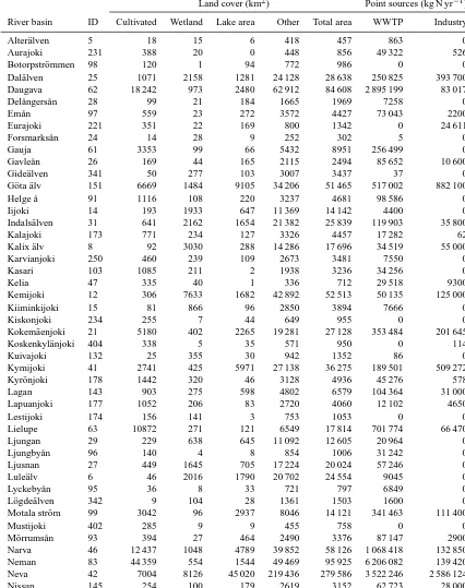
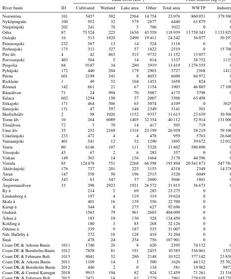
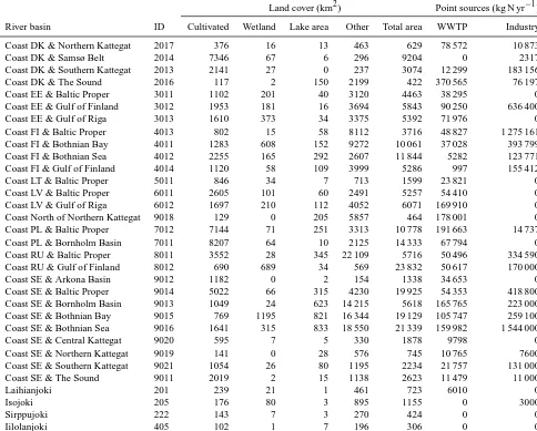
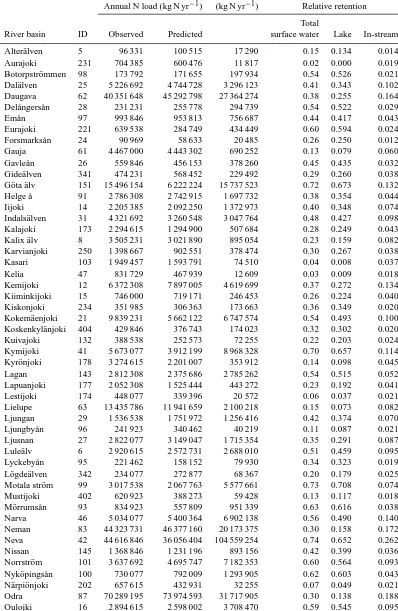
Table A1. Input data to the MESAW model for estimation of total nitrogen (N) retention. Input data include land cover (cultivated, wetland, lake area, other and total drainage area; km2) and point source emissions (WWTP and industry; kg N yr−1). Observed annual loads are given with the retention results in Table A2.

Land cover (km2) Point sources (kg N yr−1)

River basin ID Cultivated Wetland Lake area Other Total area WWTP Industry

Alterälven 5 18 15 6 418 457 863 0

Aurajoki 231 388 20 0 448 856 49 322 526

Botorpströmmen 98 120 1 94 772 986 0 0

Dalälven 25 1071 2158 1281 24 128 28 638 250 825 393 700

Daugava 62 18 242 973 2480 62 912 84 608 2 895 199 83 017

Delångersån 28 99 21 184 1665 1969 7258 0

Emån 97 559 23 272 3572 4427 73 043 2200

Eurajoki 221 351 22 169 800 1342 0 24 611

Forsmarksån 24 14 28 9 252 302 5 0

Gauja 61 3353 99 66 5432 8951 256 499 0

Gavleån 26 169 44 165 2115 2494 85 652 10 600

Gideälven 341 50 277 103 3007 3437 37 0

Göta älv 151 6669 1484 9105 34 206 51 465 517 002 882 100

Helge å 91 1116 108 220 3237 4681 98 586 0

Iijoki 14 193 1933 647 11 369 14 142 4400 0

Indalsälven 31 641 2162 1654 21 382 25 839 119 903 35 800

Kalajoki 173 771 234 127 3326 4457 17 282 62

Kalix älv 8 92 3030 288 14 286 17 696 34 519 55 000

Karvianjoki 250 460 239 109 2673 3481 7550 0

Kasari 103 1085 211 2 1938 3236 34 256 0

Kelia 47 335 40 1 336 712 29 518 9300

Kemijoki 12 306 7633 1682 42 892 52 513 50 135 125 000

Kiiminkijoki 15 81 866 96 2850 3894 7666 0

Kiskonjoki 234 255 7 44 649 955 0 0

Kokemäenjoki 21 5180 402 2265 19 281 27 128 353 484 201 645

Koskenkylänjoki 404 338 5 35 571 950 0 114

Kuivajoki 132 25 355 30 942 1352 86 0

Kymijoki 41 2741 425 5971 27 138 36 275 189 501 509 272

Kyrönjoki 178 1442 320 46 3128 4936 45 276 578

Lagan 143 903 275 598 4802 6579 104 364 31 000

Lapuanjoki 177 1052 206 83 2720 4060 12 102 4650

Lestijoki 174 156 141 3 753 1053 0 0

Lielupe 63 10872 271 121 6549 17 814 701 774 66 470

Ljungan 29 229 638 645 11 092 12 605 20 964 0

Ljungbyån 96 140 4 8 854 1006 31 242 0

Ljusnan 27 449 1645 705 17 224 20 024 57 246 0

Luleälv 6 46 2016 1790 20 702 24 554 9045 0

Lyckebyån 95 36 8 33 721 797 6849 0

Lögdeälven 342 9 104 28 1361 1503 1600 0

Motala ström 99 3042 96 2937 8046 14 121 341 463 111 400

Mustijoki 402 285 9 9 455 758 0 0

Mörrumsån 93 394 27 464 2490 3376 87 147 2900

Narva 46 12 437 1048 4789 39 852 58 126 1 068 418 132 850

Neman 83 44 359 554 1544 49 469 95 925 6 206 082 139 420

Neva 42 7004 8126 45 020 219 436 279 586 3 522 246 2 586 124

Table A1. Continued.

Land cover (km2) Point sources (kg N yr−1)

River basin ID Cultivated Wetland Lake area Other Total area WWTP Industry

Norrström 101 5457 302 2564 14 754 23 076 860 051 379 300

Nyköpingsån 100 952 32 579 2877 4440 61 879 0

Närpiönjoki 202 241 70 5 706 1022 0 0

Odra 87 73 524 225 1630 43 559 118 939 13 758 343 1 133 829

Oulojki 16 513 1828 2490 19 411 24 242 36 077 50 297

Paimionjoki 232 567 13 14 524 1118 0 0

Perhonjoki 175 313 327 57 1822 2519 0 15 700

Pite älv 4 42 863 515 9732 11 152 13 057 0

Porvoonjoki 403 504 5 14 814 1337 38 752 1135

Pregolia 84 9187 34 280 3919 13 419 1 276 555 0

Pyhäjoki 172 440 204 179 2903 3727 2568 1412

Pärnu 601 2198 341 8 4053 6600 84 972 0

Rickleån 1 49 52 104 1453 1658 824 0

Rönneå 142 661 21 67 1154 1903 46 885 17 100

Råneälven 71 24 994 70 3087 4175 3798 0

Salaca 602 1294 150 57 2007 3508 63 498

Siikajoki 171 464 506 65 3074 4109 0 3629

Simojoki 131 47 597 148 2349 3141 501 0

Skellefteälv 2 98 1026 1152 9337 11 613 23 639 30 500

Torne älv 10 264 6089 1405 32 354 40 112 52 914 131 000

Töreälven 72 3 70 14 417 505 719 0

Ume älv 35 252 2169 1318 23 199 26 939 38 219 59 100

Uskelanjoki 233 472 4 4 478 959 5763 26 640

Vantaanjoki 401 541 12 52 1290 1895 39 672 12 032

Venta 80 6146 107 111 5328 11 692 580 890 0

Vironjoki 43 67 2 6 283 357 0 0

Viskan 149 365 14 136 1664 2178 44 596 0

Vistula 85 124 478 751 2268 66 398 193 894 20 541 873 547 784

Ähtävänjoki 176 737 201 225 3155 4318 2349 14 376

Ätran 147 558 50 196 2515 3320 6049 0

Öreälven 343 63 347 37 2600 3046 1801 0

Ångermanälven 33 398 2923 1921 26 572 31 815 36 673 0

Ry å 214 2 69 285 23 275 0

Lindenborg å 197 4 119 319 19 624 0

Skals å 401 16 139 556 22 700 0

Karup å 344 8 275 627 92 696 0

Gudenå 1563 79 961 2603 404 099 0

Århus å 183 10 130 324 134 450 0

Kolding å 180 3 85 268 32 126 0

Odense å 339 9 187 535 31 007 0

Ndr. Halleby å 272 18 128 418 31 204 0

Suså 478 24 254 756 107 901 0

Coast DE & Arkona Basin 1011 1740 28 8 620 2395 74 132 0

Coast DE & Bornholm Basin 1012 7858 81 191 2455 10 585 336 061 1535

Coast DE & Fehmarn Belt 1013 8041 52 280 2148 10 522 377 142 23 830

Coast DK & Arkona Basin 2011 1109 14 3 500 1626 44 132 55 702

Coast DK & Bornholm Basin 2012 446 2 0 134 581 19 962 9873

Coast DK & Central Kattegat 2018 9915 194 82 824 12 459 71 261 21 316

Table A1. Continued.

Land cover (km2) Point sources (kg N yr−1)

River basin ID Cultivated Wetland Lake area Other Total area WWTP Industry

Coast DK & Northern Kattegat 2017 376 16 13 463 629 78 572 10 873

Coast DK & Samsø Belt 2014 7346 67 6 296 9204 0 2317

Coast DK & Southern Kattegat 2013 2141 27 0 237 3074 12 299 183 156

Coast DK & The Sound 2016 117 2 150 2199 422 370 565 76 197

Coast EE & Baltic Proper 3011 1102 201 40 3120 4463 38 295 0

Coast EE & Gulf of Finland 3012 1953 181 16 3694 5843 90 250 636 400

Coast EE & Gulf of Riga 3013 1610 373 34 3375 5392 71 976 0

Coast FI & Baltic Proper 4013 802 15 58 8112 3716 48 827 1 275 161

Coast FI & Bothnian Bay 4011 1283 608 152 9272 10 061 37 028 393 799

Coast FI & Bothnian Sea 4012 2255 165 292 2607 11 844 5282 123 771

Coast FI & Gulf of Finland 4014 1120 58 109 3999 5286 997 155 412

Coast LT & Baltic Proper 5011 846 34 7 713 1599 23 821 0

Coast LV & Baltic Proper 6011 2605 101 60 2491 5257 54 410 0

Coast LV & Gulf of Riga 6012 1697 210 112 4052 6071 169 910 0

Coast North of Northern Kattegat 9018 129 0 205 5857 464 178 001 0

Coast PL & Baltic Proper 7012 7144 71 251 3313 10 778 191 663 14 737

Coast PL & Bornholm Basin 7011 8207 64 10 2125 14 333 67 794 0

Coast RU & Baltic Proper 8011 3552 28 345 22 109 5716 50 496 334 590

Coast RU & Gulf of Finland 8012 690 689 34 569 23 832 50 617 170 000

Coast SE & Arkona Basin 9012 1182 0 2 154 1338 34 653 0

Coast SE & Baltic Proper 9014 5022 66 315 4230 19 925 54 353 418 800

Coast SE & Bornholm Basin 9013 1049 24 623 14 215 5618 165 765 223 000

Coast SE & Bothnian Bay 9015 769 1195 821 16 344 19 129 105 747 259 100

Coast SE & Bothnian Sea 9016 1641 315 833 18 550 21 339 159 982 1 544 000

Coast SE & Central Kattegat 9020 595 7 5 330 1878 9798 0

Coast SE & Northern Kattegat 9019 141 0 28 576 745 10 765 7600

Coast SE & Southern Kattegat 9021 1054 26 80 1195 2234 21 757 131 000

Coast SE & The Sound 9011 2019 2 15 1138 2623 11 479 11 000

Laihianjoki 201 239 21 1 461 723 6010 0

Isojoki 205 176 80 3 895 1155 0 3000

Sirppujoki 222 143 7 3 270 424 0 0

Table A2. Observed and predicted annual N loads (kg N yr−1) and total N retention as estimated by the MESAW model.

Retention

Annual N load (kg N yr−1) (kg N yr−1) Relative retention Total

River basin ID Observed Predicted surface water Lake In-stream

Alterälven 5 96 331 100 515 17 290 0.15 0.134 0.014

Aurajoki 231 704 385 600 476 11 817 0.02 0.000 0.019

Botorpströmmen 98 173 792 171 655 197 934 0.54 0.526 0.021

Dalälven 25 5 226 692 4 744 728 3 296 123 0.41 0.343 0.102

Daugava 62 40 351 648 45 292 798 27 364 274 0.38 0.255 0.164

Delångersån 28 231 231 255 778 294 739 0.54 0.522 0.029

Emån 97 993 846 953 813 756 687 0.44 0.417 0.043

Eurajoki 221 639 538 284 749 434 449 0.60 0.594 0.024

Forsmarksån 24 90 969 58 633 20 485 0.26 0.250 0.012

Gauja 61 4 467 000 4 443 302 690 252 0.13 0.079 0.060

Gavleån 26 559 846 456 153 378 260 0.45 0.435 0.032

Gideälven 341 474 231 568 452 229 492 0.29 0.260 0.038

Göta älv 151 15 496 154 6 222 224 15 737 523 0.72 0.673 0.132

Helge å 91 2 786 308 2 742 915 1 697 732 0.38 0.354 0.044

Iijoki 14 2 205 385 2 092 250 1 372 973 0.40 0.348 0.074

Indalsälven 31 4 321 692 3 260 548 3 047 764 0.48 0.427 0.098

Kalajoki 173 2 294 615 1 294 900 507 684 0.28 0.249 0.043

Kalix älv 8 3 505 231 3 021 890 895 054 0.23 0.159 0.082

Karvianjoki 250 1 398 667 902 551 378 474 0.30 0.267 0.038

Kasari 103 1 949 457 1 593 791 74 510 0.04 0.008 0.037

Kelia 47 831 729 467 939 12 609 0.03 0.009 0.018

Kemijoki 12 6 372 308 7 897 005 4 619 699 0.37 0.272 0.134

Kiiminkijoki 15 746 000 719 171 246 453 0.26 0.224 0.040

Kiskonjoki 234 351 985 306 363 173 663 0.36 0.349 0.020

Kokemäenjoki 21 9 839 231 5 662 122 6 747 574 0.54 0.493 0.100

Koskenkylänjoki 404 429 846 376 743 174 023 0.32 0.302 0.020

Kuivajoki 132 388 538 252 573 72 255 0.22 0.203 0.024

Kymijoki 41 5 673 077 3 912 199 8 968 328 0.70 0.657 0.114

Kyrönjoki 178 3 274 615 2 201 007 353 912 0.14 0.098 0.045

Lagan 143 2 812 308 2 375 686 2 785 262 0.54 0.515 0.052

Lapuanjoki 177 2 052 308 1 525 444 443 272 0.23 0.192 0.041

Lestijoki 174 448 077 339 396 20 572 0.06 0.037 0.021

Lielupe 63 13 435 786 11 941 659 2 100 218 0.15 0.073 0.082

Ljungan 29 1 536 538 1 751 972 1 256 416 0.42 0.374 0.070

Ljungbyån 96 241 923 340 462 40 219 0.11 0.087 0.021

Ljusnan 27 2 822 077 3 149 047 1 715 354 0.35 0.291 0.087

Luleälv 6 2 920 615 2 572 731 2 688 010 0.51 0.459 0.095

Lyckebyån 95 221 462 158 152 79 930 0.34 0.323 0.019

Lögdeälven 342 234 077 272 877 68 367 0.20 0.179 0.025

Motala ström 99 3 017 538 2 067 763 5 577 661 0.73 0.708 0.074

Mustijoki 402 620 923 388 273 59 428 0.13 0.117 0.018

Mörrumsån 93 834 923 557 809 951 339 0.63 0.616 0.038

Narva 46 5 034 077 5 400 364 6 902 138 0.56 0.490 0.140

Neman 83 44 323 731 46 377 160 20 173 375 0.30 0.158 0.172

Neva 42 44 616 846 36 056 404 104 559 254 0.74 0.652 0.262

Nissan 145 1 368 846 1 231 196 893 156 0.42 0.399 0.036

Norrström 101 3 637 692 4 695 747 7 182 353 0.60 0.564 0.093

Nyköpingsån 100 730 077 792 009 1 293 905 0.62 0.603 0.043

Närpiönjoki 202 657 615 432 931 32 255 0.07 0.049 0.021

Odra 87 70 289 195 73 974 593 31 717 905 0.30 0.138 0.188

Table A2. Continued.

Retention

Annual N load (kg N yr−1) (kg N yr−1) Relative retention

Total

River basin ID Observed Predicted surface water Lake In-stream

Paimionjoki 232 900 846 680 805 114 622 0.14 0.125 0.022

Perhonjoki 175 815 769 688 291 209 547 0.23 0.208 0.033

Pite älv 4 1 594 231 1 492 285 966 100 0.39 0.350 0.066

Porvoonjoki 403 1 303 615 723 513 107 528 0.13 0.108 0.024

Pregolia 84 4 580 143 4 207 286 1 429 755 0.25 0.195 0.072

Pyhäjoki 172 1 127 385 807 208 504 218 0.38 0.359 0.039

Pärnu 601 3 091 070 3 193 671 219 537 0.06 0.013 0.052

Rickleån 1 283 462 233 266 181 333 0.44 0.422 0.027

Rönneå 142 2 587 846 1 511 841 682 779 0.31 0.291 0.029

Råneälven 71 540 308 714 315 177 607 0.20 0.164 0.042

Salaca 602 2 287 635 1 585 606 377 174 0.19 0.160 0.038

Siikajoki 171 1 332 615 1 127 084 266 866 0.19 0.157 0.041

Simojoki 131 748 231 471 133 286 563 0.38 0.355 0.036

Skellefteälv 2 1 319 385 1 124 731 1 475 798 0.57 0.536 0.068

Torne älv 10 5 154 615 5 552 103 3 319 728 0.37 0.290 0.119

Töreälven 72 89 992 83 532 28 567 0.25 0.244 0.015

Ume älv 35 3 359 846 3 522 076 2 619 449 0.43 0.363 0.099

Uskelanjoki 233 508 182 652 521 47 115 0.07 0.048 0.020

Vantaanjoki 401 1 283 000 753 105 269 584 0.26 0.242 0.028

Venta 80 6 649 974 7 118 779 1 365 064 0.16 0.100 0.068

Vironjoki 43 213 534 122 758 26 503 0.18 0.167 0.013

Viskan 149 1 568 692 1 016 516 792 104 0.44 0.420 0.030

Vistula 85 112 041 104 116 917 897 55 292 179 0.32 0.120 0.229

Ähtävänjoki 176 419 608 1 049 732 713 541 0.40 0.378 0.042

Ätran 147 2 007 769 1 529 797 1 155 539 0.43 0.408 0.037

Öreälven 343 491 769 605 790 110 818 0.15 0.123 0.036

Ångermanälven 33 4 223 154 3 798 849 3 450 419 0.48 0.413 0.107

Ry å 537 807 495 987

Lindenborg å 724 156 458 904

Skals å 683 604 743 902

Karup å 720 306 866 486

Gudenå 3 075 608 3 177 587

Århus å 442 719 446 084

Kolding å 651 265 423 277

Odense å 1 071 416 740 493

Ndr. Halleby å 275 250 473 721

Suså 961 097 952 650

Coast DE & Arkona Basin 1011 1 953 735 139 436 0.07 0.036 0.032

Coast DE & Bornholm Basin 1012 7 394 183 2 176 860 0.23 0.174 0.065

Coast DE & Fehmarn Belt 1013 7 094 187 2 843 034 0.29 0.237 0.065

Coast DK & Arkona Basin 2011 1 345 482 61 852 0.04 0.018 0.026

Coast DK & Bornholm Basin 2012 529 791 8 593 0.02 0.000 0.016

Coast DK & Central Kattegat 2018 9 543 967 1 505 255 0.14 0.071 0.070

Coast DK & Fehmarn Belt 2015 2 715 470 783 402 0.22 0.195 0.035

Coast DK & Northern Kattegat 2017 483 611 127 542 0.21 0.195 0.017

Coast DK & Samsø Belt 2014 7,432 683 537 534 0.07 0.007 0.061

Coast DK & Southern Kattegat 2013 2 458 534 91 878 0.04 0.000 0.036

Coast DK & The Sound 2016 232 761 984 193 0.81 0.806 0.014

Coast EE & Baltic Proper 3011 1 711 747 261 982 0.13 0.094 0.043

Coast EE & Gulf of Finland 3012 3 399 885 289 177 0.08 0.031 0.049

Table A2. Continued.

Retention

Annual N load (kg N yr−1) (kg N yr−1) Relative retention

Total

River basin ID Observed Predicted surface water Lake In-stream

Coast FI & Baltic Proper 4013 3 285 098 754 614 0.19 0.153 0.039

Coast FI & Bothnian Bay 4011 3 211 420 818 564 0.20 0.149 0.063

Coast FI & Bothnian Sea 4012 2 382 056 908 814 0.28 0.223 0.068

Coast FI & Gulf of Finland 4014 1 783 711 535 861 0.23 0.193 0.047

Coast LT & Baltic Proper 5011 1 024 349 78 227 0.07 0.046 0.026

Coast LV & Baltic Proper 6011 2 919 632 550 310 0.16 0.118 0.047

Coast LV & Gulf of Riga 6012 2 347 634 656 593 0.22 0.178 0.050

Coast North of Northern Kattegat 9018 291 927 1 530 714 0.84 0.838 0.014

Coast PL & Baltic Proper 7012 6 523 722 2 349 513 0.26 0.213 0.065

Coast PL & Bornholm Basin 7011 8 603 413 770 891 0.08 0.008 0.075

Coast RU & Baltic Proper 8011 5 280 324 4 169 888 0.44 0.413 0.048

Coast RU & Gulf of Finland 8012 1 082 667 132 001 0.11 0.016 0.094

Coast SE & Arkona Basin 9012 1 284 175 55 321 0.04 0.018 0.024

Coast SE & Baltic Proper 9014 5 408 956 1 605 059 0.23 0.156 0.087

Coast SE & Bornholm Basin 9013 2 193 909 3 088 678 0.58 0.564 0.048

Coast SE & Bothnian Bay 9015 3 191 350 2 042 113 0.39 0.333 0.085

Coast SE & Bothnian Sea 9016 4 986 008 2 981 173 0.37 0.313 0.089

Coast SE & Central Kattegat 9020 687 471 41 291 0.06 0.029 0.028

Coast SE & Northern Kattegat 9019 222 276 101 656 0.31 0.301 0.018

Coast SE & Southern Kattegat 9021 1 120 775 520 464 0.32 0.295 0.031

Coast SE & The Sound 9011 2 227 338 232 256 0.09 0.063 0.033

Laihianjoki 201 356 461 13 468 0.04 0.019 0.018

Isojoki 205 385 234 21 891 0.05 0.032 0.022

Sirppujoki 222 195 592 21 695 0.10 0.087 0.014

Acknowledgements. This paper is a contribution from the RE-COCA project, which has received funding from the BONUS+ program funded jointly by the European Community’s Seventh framework Programme (FP7/2007-2013, grant agreement 217246) and Baltic Sea national funding institutions. Additional funding for the Norwegian authors was provided under the research grant AGRI-LOSS of the Norwegian Research Council. This work was, for the Estonian co-author, also supported by institutional research funding IUT (IUT19-17) of the Estonian Ministry of Education and Research. We thank the two anonymous reviewers for their constructive comments, which helped to improve the manuscript.

Edited by: A. D. Reeves

References

Alexander, R. B., Smith, R. A., and Schwarz, G. E.: Effect of stream channel size on the delivery of nitrogen to the gulf of Mexico, Nature, 403, 758–761, 2000.

Behrendt, H. and Opitz, D.: Retention of nutrients in river systems: dependence on specific runoff and hydraulic load, Hydrobiolo-gia, 410, 111–122, 2000.

Bergström, S. and Carlsson, B.: River runoff to the Baltic Sea – 1950–1990, Ambio, 23, 280–287, 1994.

Billen, G., Thieu, V., Garnier, J., and Silvestre, M.: Modelling the N cascade in regional watersheds: The case study of the Seine, Somme and Scheldt rivers, Agr. Ecosyst. Environ., 133, 234– 246, 2009.

Grimvall, A. and Stålnacke, P.: Statistical methods for source ap-portionment of riverine loads of pollutants, Environmetrics, 7, 201–213, 1996.

Harrison, J. A., Maranger, R. J., Alexander, R. B., Giblin, A. E., Jacinthe, P. A., Mayorga, E., Seitzinger, S. P., Sobota, D. J., and Wollheim, W. M.: The regional and global significance of nitro-gen removal in lakes and reservoirs, Biogeochemistry, 93, 143– 157, 2009.

Hejzlar, J., Anthony, S., Arheimer, B., Behrendt, H., Bouraoui, F., Grizzetti, B., Groenendijk, P., Jeuken, M., Johnsson, H., Lo Porto, A., Kronvang, B., Panagopoulos, Y., Siderius, C., Silgram, M., Venohr, M., and Zaloudik, J.: Nitrogen and phosphorus re-tention in surface waters: an inter-comparison of predictions by catchment models of different complexity, J. Environ. Monitor., 11, 584–593, 2009.

HELCOM: The fifth Baltic Sea pollution load compilation (PLC-5), Baltic Marine Environment Protection Commission, Baltic Sea Environment Proceedings No. 128, Helsinki Commission, Helsinki, Finland, 2011.

Hesse, C., Krysanova, V., Vetter, T., and Reinhardt, J.: Comparison of several approaches representing terrestrial and in-stream nutri-ent retnutri-ention and decomposistion in watershed modelling, Ecol. Modell., 269, 70–85, 2013.

Hill, B. H. and Bolgrien, D. W.: Nitrogen removal by streams and rivers of the Upper Mississippi River basin, Biogeochemistry, 102, 183–194, 2011.

Hoffmann, C. C., Kjaergaard, C., Uusi-Kamppa, J., Hansen, H. C. B., and Kronvang, B.: Phosphorus Retention in Riparian Buffers: Review of Their Efficiency, J. Environ. Quality, 38, 1942–1955, 2009.

Jeppesen, E., Kronvang, B., Olesen, J. E., Audet, J., Sondergaard, M., Hoffmann, C. C., Andersen, H. E., Lauridsen, T. L., Libo-riussen, L., Larsen, S. E., Beklioglu, M., Meerhoff, M., Ozen, A., and Ozkan, K.: Climate change effects on nitrogen loading from cultivated catchments in Europe: implications for nitrogen retention, ecological state of lakes and adaptation, Hydrobiolo-gia, 663, 1–21, 2011.

Jordan, S. J., Stoffer, J., and Nestlerode, J. A.: Wetlands as Sinks for Reactive Nitrogen at Continental and Global Scales: A Meta-Analysis, Ecosystems, 14, 144–155, 2011.

Jung, H. S. and Deng, Z. Q.: Modeling of Nitrogen Retention in Amite River, Water Air Soil Poll., 215, 411–425, 2011. Kellogg, D. Q., Gold, A. J., Cox, S., Addy, K., and August, P. V.:

A geospatial approach for assessing denitrification sinks within lower-order catchments, Ecol. Eng., 36, 1596–1606, 2010. Lidèn, R., Vassiljev, A., Loigu, E., Stålnacke, P., and Wittgren, H.

B.: Nitrogen source apportionment using a physically and statis-tically based model, Ecol. Modell., 114, 235–250, 1999. Mayorga, E., Seitzinger, S. P., Harrison, J. A., Dumont, E., Beusen,

A. H. W., Bouwman, A. F., Fekete, B. M., Kroeze, C., and Van Drecht, G.: Global Nutrient Export from WaterSheds 2 (NEWS 2): Model development and implementation, Environ. Modell. Softw., 25, 837–853, 2010.

Mörth, C. M., Humborg, C., Eriksson, H., Danielsson, A., Medina, M. R., Lofgren, S., Swaney, D. P., and Rahm, L.: Modeling river-ine nutrient transport to the Baltic Sea: A large-scale approach, Ambio, 36, 124–133, 2007.

Mulholland, P. J., Helton, A. M., Poole, G. C., Hall, R. O., Hamil-ton, S. K., Peterson, B. J., Tank, J. L., Ashkenas, L. R., Cooper, L. W., Dahm, C. N., Dodds, W. K., Findlay, S. E. G., Gregory, S. V., Grimm, N. B., Johnson, S. L., McDowell, W. H., Meyer, J. L., Valett, H. M., Webster, J. R., Arango, C. P., Beaulieu, J. J., Bernot, M. J., Burgin, A. J., Crenshaw, C. L., Johnson, L. T., Niederlehner, B. R., O’Brien, J. M., Potter, J. D., Sheibley, R. W., Sobota, D. J., and Thomas, S. M.: Stream denitrification across biomes and its response to anthropogenic nitrate loading, Nature, 452, 202–205, 2008.

Povilaitis, A., Stålnacke, P., and Vassiliev, A.: Nutrient retention and export to surface waters in Lithuanian and Estonian river basins, Hydrol. Res., 43, 359–373, 2012.

Seitzinger, S. P.: Nitrogen cycle – Out of reach, Nature, 452, 162– 163, 2008.

Seitzinger, S. P., Styles, R. V., Boyer, E. W., Alexander, R. B., Billen, G., Howarth, R. W., Mayer, B., and Van Breemen, N.: Ni-trogen retention in rivers: model development and application to watersheds in the northeastern USA, Biogeochemistry, 57, 199– 237, 2002.

Seitzinger, S. P., Harrison, J. A., Böhlke, J. K., Bouwman, A. F., Lowrance, R., Peterson, B., Tobias, C., and Drecht, G. V.: Deni-trification across landscapes and waterscapes: A synthesis, Ecol. Appl., 16, 2064–2090, 2006.

Smith, R. A., Schwarz, G. E., and Alexander, R. B.: Regional inter-pretation of water-quality monitoring data, Water Resour. Res., 33, 2781–2798, 1997.

Stålnacke, P., Aakerøy, P.A., Blicher-Mathiesen, G., Iital, A., Jan-sons, V., Koskiaho, J., Kyllmar, K., Lagzdins, A., Pengerud, A., and Povilaitis, A.: Temporal trends in nitrogen concentrations and losses from agricultural catchments in the Nordic and Baltic countries, Agricult. Ecosys. Environ., 198, 94–103, 2014. Vassiljev, A. and Stålnacke, P.: Source apportionment of nutrients

in the Lake Peipsi drainage basin – experiences from a statistical model, Water Sci. Technol., 51, 309–317, 2005.

Vassiljev, A., Blinova, I., and Ennet, P.: Source apportionment of nutrients in Estonian rivers, Desalination, 226, 222–230, 2008. Wollheim, W. M., Voosmarty, C. J., Peterson, B. J., Seitzinger,