Wouter Greuell, Wietse H. P. Franssen, and Ronald W. A. Hutjes
Water Systems and Global Change (WSG) group, Wageningen University and Research, Droevendaalsesteeg 3, 6708 PB Wageningen, the Netherlands
Correspondence:Wouter Greuell ([email protected])
Received: 17 November 2016 – Discussion started: 30 November 2016
Revised: 28 November 2018 – Accepted: 21 December 2018 – Published: 22 January 2019
Abstract. This paper uses hindcasts (1981–2010) to inves-tigate the sources of skill in seasonal hydrological forecasts for Europe. The hindcasts were produced with WUSHP (Wa-geningen University Seamless Hydrological Prediction sys-tem). Skill was identified in a companion paper. In WUSHP, hydrological processes are simulated by running the Vari-able Infiltration Capacity (VIC) hydrological model forced with an ensemble of bias-corrected output from the seasonal forecast system 4 (S4) of the European Centre for Medium-Range Weather Forecasts (ECMWF). We first analysed the meteorological forcing. The precipitation forecasts contain considerable skill for the first lead month but hardly any sig-nificant skill at longer lead times. Seasonal forecasts of tem-perature have more skill. Skill in summer temtem-perature is re-lated to climate change and is more or less independent of lead time. Skill in February and March is unrelated to climate change. Different sources of skill in hydro-meteorological variables were isolated with a suite of specific hydrologi-cal hindcasts akin to ensemble streamflow prediction (ESP). These hindcasts show that in Europe, initial conditions of soil moisture (SM) form the dominant source of skill in run-off. From April to July, initial conditions of snow contribute sig-nificantly to the skill. Some remarkable skill features are due to indirect effects, i.e. skill due to forcing or initial condi-tions of snow and soil moisture at an earlier stage is stored in the hydrological state (snow and/or soil moisture) of a later stage, which then contributes to persistence of skill. Skill in evapotranspiration (ET) originates mostly in the meteorolog-ical forcing. For run-off we also compared the full hindcasts (with S4 forcing) with two types of ESP (or ESP-like) hind-casts (with identical forcing for all years). Beyond the second lead month, the full hindcasts are less skilful than the ESP (or
ESP-like) hindcasts, because inter-annual variations in the S4 forcing consist mainly of noise which enhances degradation of the skill.
1 Introduction
Society may benefit from seasonal hydrological forecasts (Viel et al., 2016; Soares and Dessai, 2016; Crochemore et al., 2016), i.e. hydrological forecasts for future time periods from more than 2 weeks up to about a year (Doblas-Reyes et al., 2013). Such predictions can be exploited to optimise, for example, hydropower energy generation (Hamlet et al., 2002), navigability of rivers in low flow conditions (Li et al., 2008) and irrigation management (Ghile and Schulze, 2008; Mushtaq et al., 2012) to decrease crop yield losses.
This is the second paper about seasonal hydrological fore-casts for Europe produced with WUSHP (Wageningen Uni-versity Seamless Hydrological Prediction system), a dynam-ical (i.e. model-based) system. In summary, the forecasts of WUSHP are made with the Variable Infiltration Capacity (VIC) hydrological model, which uses bias-corrected output of forecasts from the seasonal forecasting system 4 (S4) of the European Centre for Medium-Range Weather Forecasts (ECMWF) as meteorological forcing. The system is proba-bilistic.
Sig-mained even at the end of the hindcasts (7 months).
To extend the evaluation of the system, its reliability was analysed. The main finding is that during the 2 first lead months the system is not far from being perfectly reliable but that with progressing lead time reliability is reduced. We also found that discrimination skill and reliability have simi-lar characteristics, e.g. for longer lead times the highest val-ues of reliability are found in some regions with considerable amounts of discrimination skill. Details of this analysis are provided in Appendix A.
The current paper aims to identify the sources of the skill in WUSHP and is structured in two main parts. In the first part, an analysis of the skill in the most important meteoro-logical forcing variables (precipitation, 2 m temperature and incoming short-wave radiation from S4) is presented. For S4, this was done earlier by Kim et al. (2012) for the boreal win-ter months (DJF), with initialisation on the first of November. For that case, they found that in Europe, S4 has no skill in the precipitation forecasts and some skill in the temperature forecasts for southern Sweden, southern Finland, the region southeast of Saint Petersburg and northern Germany. Scaife et al. (2014) analysed the skill for the same target months and starting date but with another prediction system, namely the Met Office Global Seasonal Forecast System version 5 (GloSea5). They found that, while the GloSea5 tempera-ture forecasts for Europe contain hardly any significant skill, the GloSea5 forecasts of the North Atlantic Oscillation are correlated significantly with observed temperatures in north-ern and southnorth-ern Europe. This means that there is untapped predictability in the GloSea5 temperature forecasts. We will analyse predictability of the mentioned output variables of S4 for the whole continent and will consider all combinations of lead and target months.
The second line of analysis aims to investigate the reasons for the presence or absence of skill in hydro-meteorological variables by means of a series of specific hindcasts that iso-late potential sources of skill, namely meteorological forc-ing, the initial conditions of soil moisture (SM) and the ini-tial conditions of snow. Such an approach was explored ear-lier by Wood et al. (2005), Bierkens and van Beek (2009) and Koster et al. (2010). Each specific hindcast is basically identical to the standard hindcasts that we analysed in the companion paper, named full streamflow hindcasts (Full-SHs; climate-model-based hindcasts” according to Yuan et al., 2015). However, in the specific hindcasts, one or two
our specific hindcasts, be used to isolate sources of skill. The main difference between the specific hindcasts of this study and the ESP technique is that in ESP and its variant reverse ESP, the meteorological forcing is taken from data based on observations, while in the present study the forcing is taken from meteorological hindcasts. In fact, we also pro-duced ESP. In Sect. 4.3 we will compare these with one of the other specific hindcasts and discuss the relation between our specific hindcasts and the ESP suite more generally.
Though this paper focusses on run-off, the analysis is com-plemented with an analysis of the skill in evapotranspiration (ET), since this variable has a large effect on run-off (see Willmott et al., 1985). Predictions of evapotranspiration also have independent value, because they are useful for planning of water level control in polders and for planning of water use for irrigation and fertiliser application. As for run-off, we will exploit the specific hindcasts to isolate the different sources of predictability in evapotranspiration forecasts.
The version of VIC that we used was only crudely cali-brated (Nijssen et al., 2001). Hence, discharge computed by the present version of the system may be expected to deviate substantially from observations, both in terms of the mean and in terms of the spread of the ensemble of forecasts. Also, within WUSHP no post-processing of discharge is carried out to correct for such deficiencies. This makes the system unsuitable for issuing forecasts of absolute amounts of dis-charge, but the system can be used to provide information on how likely it is that the future discharge will be above or below normal. Consequently, the most important criteria for the selection of skill metrics (see Sect. 2.2) are their ability of discrimination and their insensitivity to biases and to the spread of the forecasts.
bers), so each set of hindcasts consists of a total of 5400 runs (30 years×12 months×15 members). In addition a single reference simulation was performed in which VIC was run with a gridded data set of model-assimilated meteorological observations, namely the WATCH Forcing Data Era-Interim (WFDEI; Weedon et al., 2014). The reference simulation has a dual aim. The first aim is to create initialisation states for the hindcasts. Secondly, the output of the reference simula-tion, e.g. run-off, is used for verification of the hindcasts. This output will be named “pseudo-observations” here.
Due to the set-up of the routing module of VIC, the state of discharge could not be saved and loaded. Hence for spin-up discharge, each 7-month hindcast was preceded by a 1-month simulation with WFDEI forcing, which in turn was initialised with the model states generated in the reference simulation and zero discharge. All hindcasts and simulations were performed on a 0.5◦×0.5◦grid in natural flow mode, i.e. river regulation, irrigation and other anthropogenic influ-ences were not considered. VIC is run with a time step of 3 h. More details about the set-up of the system and the hindcasts can be found in the companion paper (Greuell et al., 2018). 2.2 Methods of analysis and observations
In this paper we analyse hindcasts of run-off, discharge and evapotranspiration. Run-off is defined as the amount of water leaving the model soil either, along the surface or at the bot-tom, while we define discharge as the flow of water through the largest river in each grid cell.
Discrimination skill (briefly skill from now on) is mea-sured in terms of the correlation coefficient between the median of the hindcasts and the observations (or pseudo-observations; R). We will designateR values as significant for pvalues less than 0.05. We also considered metrics de-signed for the evaluation of categorical forecasts (terciles), namely the relative operating characteristics (ROC) area and the ranked probability skill score (RPSS). The thresholds used for assigning individual (pseudo-)observations to ter-ciles were determined from the (pseudo-)observations them-selves. Similarly hindcasts were assigned to terciles by ref-erence to themselves. Due to this strategy metrics are unaf-fected by biases, a desired property (see Sect. 1). In the
com-the determination of com-the skill of com-the meteorological forcing we used the WFDEI data.
To investigate the possible contribution of trends to skill, skill in the meteorological forcing and in run-off was deter-mined both before and after removing the trend from both the (pseudo-) observations and the hindcasts. Data were de-trended by first constructing time series (1981–2010) for each variable, target month, lead month and grid cell (30 val-ues). We then removed the trend from each time series by first fitting a least-squares regression line to the time series and then subtracting the time series corresponding to the line from the original data. For the hindcasts, time series were constructed for the mean of the ensembles, and the resulting best fit was subtracted from each member individually.
Like in the companion paper, skill was analysed on a monthly and not on a seasonal basis with the aim of achiev-ing a relatively high temporal resolution in the skill analysis. Attention was confined to consistent skill, which we define as skill that persists during at least two consecutive target or lead months. In accordance with Hagedorn et al. (2005), we designated the first month of the hindcasts as lead month zero.
In most result sections, we will first analyse and explain skill at the level of the entire domain. We will then take out the most noteworthy details of the summary plots and seek an explanation for them.
2.3 Isolation of sources of skill and surface water initialisation
As already pointed out in the introduction, a number of spe-cific hindcasts were carried out with the aim of isolating the contributions of different sources to skill. The FullSHs, in which skill is due to both meteorological forcing and initial conditions, constitute the starting point. The specific hindcasts can be seen as restricted, in the sense of limiting the types of sources of skill, versions of the FullSHs. The following five sets of specific hindcasts, each consisting of 5400 computer runs, were produced:
con-ditions of soil moisture only. The SMInitSHs are iden-tical to the InitSHs, but in all SMInitSHs snow initial conditions are taken as the 30-year average of the snow conditions in the reference simulation.
3. TheSnInitSHsisolate the skill due to the initial condi-tions of snow contained in the snow cover. The SnInit-SHs are identical to the InitSnInit-SHs, but in all SnInitSnInit-SHs soil moisture initial conditions are taken as the 30-year average of the soil moisture conditions in the reference simulation.
4. TheMeteoSHsisolate the skill due the meteorological forcing and as such are the full complement of the Init-SHs. Like in the FullSHs, the annually varying forcing is taken from the probabilistic S4 hindcasts, while for each year the initial soil moisture and snow conditions are identical and equal to the 30-year average of the soil moisture and snow conditions in the reference simula-tion. By taking identical initial conditions for all of the years of the hindcasts, skill due to the initial conditions of soil moisture and snow is eliminated.
5. TheESPare identical to the InitSHs, both in terms of their construction and in terms of their purpose. How-ever, in the ESP the forcing is not taken from the S4 hindcasts but from the WFDEI data by selecting the 15 odd years from 1981 to 2009.
Forcings and initial conditions of all of these hindcasts dif-fer among the calendar months so that the annual cycle is conserved. Hence, in the list above, the following apply:
– “Identical for all years” means that the forcings (or the initial conditions) for all hindcasts starting in, for exam-ple, May are identical.
– “30-year average” means that the initial conditions for all hindcasts starting in, for example, May are averaged over all of the 1 May model states in the reference sim-ulation.
– “Annually varying” means that the forcings (or the ini-tial conditions) for all hindcasts starting in, for example, May vary from year to year.
These statements also hold for the other calendar months.
Discharge initialisation, a potential source of skill, is not considered. This has no effect on most of the analyses of the paper, since these are made in terms of run-off. Where dis-charge is analysed the effect of disdis-charge initialisation is, due to the limited residence time of water in the rivers, restricted to the first lead month of the hindcasts (see Yuan, 2016).
3 Explanations of skill in hydrological variables 3.1 Skill in the meteorological forcing after bias
correction
In this sub-section, the skill of the meteorological forcing will be analysed. Attention will be limited to the three in-put variables of VIC that have the largest effect on run-off and evapotranspiration, namely precipitation, 2 m tempera-ture and incoming short-wave radiation. The WFDEI data are used as a reference. Here the data after bias correction are considered. In Appendix B we will discuss the skill of the raw S4 data, which is the meteorological forcing before bias correction. Differences in skill between the bias-corrected and the uncorrected data are negligible for temperature and short-wave radiation and small for precipitation.
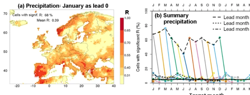
Figure 1.Skill of the precipitation hindcasts after bias correction. Figure 1a shows a map of the correlation coefficient between the observa-tions and the median of the hindcasts (R), for target month January as lead month 0. The threshold of significant skill lies at 0.31, so cells with the lightest yellow colour have insignificant skill, and grid cells with other colours have significant skill. The legend provides the percentage of cells with significant values ofRand the domain-averaged value ofR. Figure 1b depicts the percentage of cells with significant skill in terms ofRas a function of the target and lead month. Each coloured curve represents the hindcasts starting in a single month of the year and has a length of 7 (lead) months. For better visualisation the parts of the curves that end in the next year are shown twice, namely at the left-hand and the right-hand side of the graph. Black lines connect the results for identical lead times, which are specified in the legend (lead m=lead month). The horizontal line gives the expected fraction of cells with significant skill due to chance in the case that the hindcasts have no skill at all (5 %).
and mostly to coastal regions (see Fig. 1a), suggesting them to be linked to the initial state of the sea surface temperature. Figure 2 shows important aspects of skill in the 2 m tem-perature hindcasts. One aspect is the possible contribution of a 30-year trend, which could be related to greenhouse warm-ing, to the skill. Figure 2a and b provide summaries of the skill of the un-detrended and the detrended data, respectively, whereas Fig. 2c compares these two types of data. For lead month 0, the hindcasts have significant skill in the largest part of the domain (Fig. 2a and b), and detrending has a small ef-fect (Fig. 2c). At longer lead times, the percentage of cells with significant skill quickly drops towards the theoretical no-skill limit (5 %), but there are a few exceptions, namely the following:
– For lead month 1, February and March temperatures are predicted with significant skill in a considerable part of the domain (44 % in February; 53 % in March). In both months the region with skill is more or less contigu-ous and comprises the Russian part of the domain, the Ukraine and the regions bordering the southern part of the Baltic Sea (Fig. 2d and e). In February the region of skill extends towards central Europe. In March it also comprises northern Fennoscandia. This skill hardly di-minishes by detrending the data (Fig. 2b and c), sug-gesting that the skill is not related to climate change. Indeed, in February and March the observed trend (in the WFDEI data set) is insignificant across most of the domain (11 % of the domain in February and 18 % in March), and, more importantly here, it is insignifi-cant in the regions with signifiinsignifi-cant skill in the temper-ature hindcasts (Fig. 2g demonstrates this for March).
We conclude that the temperature skill in February and March as lead month 1 must be due to initial conditions of the climate model (see also the discussion on Fig. 10). – The 3 summer months (JJA) exhibit significant skill at all lead times in much more than 5 % of the do-main (a range from 22 % to 56 % for all combinations of the 3 summer months and all lead months beyond lead month 0; see Fig. 2a). In this case the fraction of cells with significant skill is not a function of lead time, which is the type of behaviour that Yuan (2016) also found for the Yellow River basin. Since Fig. 2b and c demonstrate that the skill for JJA more or less vanishes when the temperature hindcasts and observations are detrended, we conclude that the skill for these months is due to trends in the data and is hence probably related to greenhouse warming. Another conclusion is that skill that hardly varies with lead time may be related to cli-mate change.
Figure 2.Skill of the 2 m temperature hindcasts after bias correction.(a)and(b)give the percentage of cells with significant values ofRfor the un-detrended(a)and the detrended(b)temperature hindcasts (see Fig. 1b for further explanation).(c)compares annual cycles of skill of un-detrended and detrended data for the first 3 lead months. The three panels in the middle row show maps ofRfor the un-detrended temperature hindcasts for target months February(d)and March(e)as lead month 1 and July as lead month 5(f). The bottom three panels depict the correlation coefficient of the trend (not the trend itself) of the observed monthly mean temperature, for March(g)and July(i), and mean of the hindcasted temperature for July as lead month 5(h).
of the year, on average. Similarly, observed trends are significant during the 3 summer months in 67 % of the domain, versus only 24 % of the domain in the other months of the year, on average. These percentages also show that significant trends occur in a larger part of the domain in the hindcasts than in the observations. So the observations, and not the hindcasts, are mostly limiting the occurrence of trend-related skill in the temperature hindcasts. This point is illustrated by the example of July as lead month 5 in Fig. 2f, h and i, but a simi-lar illustration could have been provided for the other summer months and different lead months. Figure 2h shows that the trends of the hindcasts for July are sig-nificant across almost the entire domain (99 % of the do-main). However, according to Fig. 2i only 69 % of the domain has a significant trend in the observed July tem-peratures. Indeed, the patterns of significance of Fig. 2f (skill in the temperature hindcasts) and Fig. 2i (signifi-cance of observed trends) agree to a large extent.
– April, May and September combine the behaviour of February and March, which have skill due to initial con-ditions of the climate model, with the skill of the sum-mer months, which show skill related to trends (Fig. 2c). – January has a considerable amount of significant skill but only for lead month 2 (42 % across the domain). This skill occurs in a piece of land reaching from Eng-land to Russia, which vaguely coincides with the region in which Kim et al. (2012) found skill in the S4 tem-perature hindcasts for the 3 winter months. However, as this skill is not found in adjacent lead and target months and is thus not consistent, we speculate that this skill is spurious.
Figure 3.Skill of the incoming short-wave radiation hindcasts after bias correction.(a)gives the percentage of cells with significant values ofR(see Fig. 1b for further explanation).(b)compares annual cycles of skill of un-detrended and detrended data for the first 3 lead months (seecfor further explanation).
March to September tend to have more skill than the other months of the year. Beyond lead month 0, skill settles around the no-skill line, except from April to July, but the fraction of cells with significant skill never exceeds 21 % (in May as lead month 1). Trends in the data hardly affect skill (Fig. 3b). 3.2 Sources of skill in run-off and discharge
In these sub-section analyses the effects of the meteorologi-cal forcing and the initial conditions on the predictability of run-off and discharge (discharge is only considered in Fig. 4) are isolated. We first address the question of how much of the skill in the run-off hindcasts is linked to trends. To examine this question, the pseudo-observations and the hindcasts of run-off were detrended, and the skill was compared to that of the un-detrended data sets. We found that for lead month 2 and averaged over all months of the year, the fraction of cells with a significant R decreased from 58.7 % to 57.4 % due to detrending, a difference of 1.3 %. This difference is much smaller than the decrease for temperature (11.8 %). We con-clude that trends contribute very little to skill in run-off. All analyses of this sub-section hereafter pertain to un-detrended data.
3.2.1 The relative importance of initial hydrological conditions
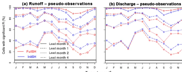
Figure 4 compares the InitSHs with the FullSHs in terms of the fraction of cells with a significantRfor run-off (Fig. 4a) and discharge (Fig. 4b). While the lumped results hardly differ between run-off and discharge (the companion paper discusses small differences in skill between these two vari-ables), systematic differences in skill between the FullSHs and InitSHs are revealed. For lead month 0, skill is higher in the FullSHs than in the InitSHs for all target months of the year, though the difference becomes very small when the fraction of the domain with significant skill approaches
100 % and hence becomes unsuitable to discriminate be-tween the two cases. Beyond lead month 1, the reverse occurs for most target months. Lead month 1 is transitional, with the order of skill depending on the time of the year. We produced figures similar to Fig. 4, all shown in the Supplement, for the skill evaluation of the following:
1. discharge with real, instead of pseudo-, observations, both for large basins (Fig. S1a in the Supplement) and small catchments (Fig. S1b) and for a subset of the large catchments with relatively little human impact (Fig. S2), 2. run-off in terms of the fraction of the domain with sig-nificant skill for the other metrics considered (RPSS, ROC above normal – AN – and ROC below normal (BN); Figs. S3–S5) and in terms of the domain-mean value ofR(Fig. S6).
In all of these cases, the reversal of skill around lead month 1 was found. So the reversal is a robust feature and is neither an artefact due to the type of observations nor due to human impacts on river flow, nor is it an artefact of the metric used in the verification procedure.
Figure 4.Comparison of the annual cycles of skill of the InitSHs (blue) and the FullSHs (red). The two panels show theoretical skill obtained with the pseudo-observations for run-off(a)and discharge(b)at four different lead times.
Figure 5.Comparison of the annual cycles of the skill in the run-off hindcasts of four specific hindcasts for lead months 0 and 2. Differ-ent colours correspond to differDiffer-ent specific hindcasts, and differDiffer-ent line types to different lead months.
different years of the run-off forecasts. If the FullSH forc-ings contain skill, these changes in ranking tend to bring, statistically, the forecasts towards the observations, so skill is added to the run-off forecasts. This is what happens at short lead times. At longer leads, the FullSHs can be considered as having no skill. This tends to randomly shuffle the ranking of the run-off forecasts and hence diminishes their skill. Of course, the ranking of the (pseudo-)observations of different years also changes during the course of the forecasts, which generally has a negative effect on run-off skill unless forc-ing is perfect. This “observation argument” complicates the whole argument but it has no consequences for the argument above, since it affects the skill of the FullSHs and the InitSHs in the same way.
3.2.2 The relative contributions of soil moisture and snow initial conditions and of meteorological forcing
Figure 5 compares the skill in run-off of the specific hind-casts (except ESP) for 2 lead months (0 and 2). At both lead times and for all target months, initialisation of soil mois-ture is the dominant source of skill in Europe. Initialisation of snow and meteorological forcing are less important. This is true for all lead times (not shown here).
tical for these months. The rapid rise in skill due to snow initialisation at the transition from April to May explains a remarkable feature that we noticed in the companion paper, namely an increase in run-off skill with lead time at this time of year. Another noticeable feature is that the skill due to snow initialisation for lead month 2 exceeds skill due to snow initialisation for lead month 0. This occurs for target months from May to August and will be explained in the text corre-sponding to Fig. 8.
Figures similar to Fig. 5, but for all metrics of the present study, are included in the Supplement (Fig. S7). The graphs for the ROC areas for the AN and BN terciles are quali-tatively similar to the graph for R. This also holds for the RPSS though fractions of the domain with significant RPSS are almost always lower than for the other metrics, probably because the RPSS is a summary metric for all three terciles including the middle one, which generally has much lower ROC areas than the other two terciles.
Figure 6 compares skill maps for the three specific hind-casts that isolate skill due to initial conditions (InitSHs, SMInitSHs and SnInitSHs). It illustrates that skill due to snow and soil moisture initialisation is not only more or less additive at the scale of the entire domain (Fig. 5) but also at the regional scale. The patterns of skill due to soil mois-ture initialisation, e.g. in Africa, on the Iberian Peninsula and in western France (Fig. 5a), are also found in the map of skill due to both components of initialisation (Fig. 5c). Small regions with considerable skill due to snow initial-isation (Fig. 5b), like those near Stockholm, in southeast-ern Czechia and southeastsoutheast-ern Austria also stick out as foci of skill on the map of skill due to both soil moisture and snow initialisation (Fig. 5c). Where both soil moisture and snow initialisation cause moderate skill, e.g. in southern Fin-land, the combined specific hindcast exhibits more signifi-cant skill.
Figure 7 zooms in on the specific hindcast that isolates skill due to snow initialisation (SnInitSHs), giving the exam-ple of a time series of skill as a function of lead time, after initialisation on 1 March. One observation is that skill does not gradually decrease with time but has a maximum dur-ing the snowmelt season. We like to note that locally skill is hardly generated during the part of the melt season when
gionally and with elevation, which largely explains the pat-terns of skill visible in the maps of Fig. 7. A good example is Scandinavia, where the earliest skill (in April; lead month 1) occurs at low elevations near the coasts of southern Nor-way and Sweden, at the end of the local snow season. The latest skill (in July; lead month 4) occurs in the Norwegian mountains, again at the end of the local snow season (we ascribe the skill in southeastern Sweden in July and August to chance). It is also relevant to note that the skill patterns in the maps of Fig. 7 are influenced by the fact that VIC has higher vertical resolution than its horizontal resolution may suggest by performing calculations in multiple elevation bands within each grid cell. This way sub-grid variations in topography are accounted for. Therefore, sub-grid topogra-phy leads to spreading of the snow skill signal of individual cells over longer periods of time.
To finish the analysis of the SnInitSHs, Fig. 8 analyses a noticeable feature. In SnInitSHs, hindcasts for May have less skill when the hindcasts are initialised on 1 May (Fig. 8a) compared to initialisation during preceding months (Febru-ary, March or April; Fig. 8b is for initialisation on 1 April). Similar results are found for June and July as target months. This result is noteworthy, because in hindcasts with initialisa-tion on 1 May, there is, due to the use of pseudo-observainitialisa-tions for verification, perfect knowledge about snow conditions on that date. With initialisation on 1 April, snow conditions on 1 May differ from those of the pseudo-observations, which by itself must lead to less skill in May run-off. The simple ex-planation is that on 1 April more grid cells have a snow cover than a month later on 1 May, but then the question arises of why those grid cells that lose their snow cover in April still exhibit significant skill in run-off during the month of May. The answer lies in an indirect effect. Inter-annual variations in the amount of snow at 1 April lead to predictable inter-annual variations in soil moisture on 1 May (Fig. 8c), when the snow cover has melted, which then acts by itself as an additional source of skill in run-off in May.
Figure 6.Example that compares the skill in run-off of three specific hindcasts (SMInitSHs –a, SnInitSHs –band InitSHs –c), for target month May as lead month 2. For more explanation, see Fig. 1a. White, terrestrial cells correspond to cells where observations or hindcasts consist for more than one-third of zeros or one-sixth of ties.
Figure 7.Example showing the variation of skill in run-off as a function of lead time in the SnInitSHs, for initialisation on 1 March. For more explanation, see Figs. 1a and 6.
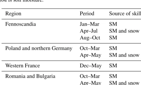
Fig. 6, for example) for three specific hindcasts that isolate the different sources of skill (SMInitSHs, SnInitSHs and Me-teoSHs). If the hotspot was present in, for example, SMInit-SHs, soil moisture initialisation is one of the sources of skill. Results are summarised in Table 1. Almost all of the signifi-cant skill in the hotspot regions is due to the initial conditions of soil moisture. Exceptions are formed by the target months from April to July, when skill is caused by a mix of the initial conditions of snow and soil moisture in regions with signif-icant snowmelt. In these cases the relative contributions of the two sources varies in time and space, but soil moisture is more important than snow, except in Fennoscandia, where snow dominates in June, and in July both sources are of about equal importance. Meteorological forcing contributed signif-icantly to this in none of the hotspots of skill.
3.3 Skill and source of skill in evapotranspiration
This section analyses skill in the hindcasts of evapotran-spiration, because hindcasts of evapotranspiration are use-ful in themselves and evapotranspiration affects run-off (see Sect. 1), and in order to demonstrate the rich possibilities of the pseudo-observations, the specific hindcasts and the detrending to unravel the various sources of skill. In VIC, evapotranspiration is computed with the Penman–Monteith method (see Shuttleworth, 1993).
[image:10.612.43.546.241.482.2]the explanation for the mechanism causing the increase in skill with lead time. For more explanation, see Figs. 1a and 6.
Figure 9.Summary plots of the skill of the hindcasts of evapotranspiration.(a)summarises the FullSHs (for more explanation, see Fig. 1b),
(b)depicts the annual cycles of skill for the FullSHs and three specific hindcasts (SnInitSHs, SMInitSHs and MeteoSHs), for lead months 0 and 2, and(c)compares the annual cycles of skill of the un-detrended and the detrended FullSHs for the first 3 lead months.
Table 1. Sources of skill for hotspot regions and periods of skill. SM is soil moisture.
Region Period Source of skill
Fennoscandia Jan–Mar SM
Apr–Jul SM and snow Aug–Oct SM
Poland and northern Germany Oct–Mar SM
Apr–May SM and snow
Western France Dec–May SM
Romania and Bulgaria Oct–Mar SM
Apr–May SM and snow Southern Mediterranean Jun–Aug SM
showing the skill for the FullSHs and three specific hindcasts. Averaged over the year, meteorological forcing (MeteoSHs) contributes more to predictability in evapotranspiration than the initial conditions, among which soil moisture (SMInit-SHs) causes more skill than snow (SnInit(SMInit-SHs). Hence, com-paring skill in run-off with skill in evapotranspiration, the
most important source of skill shifts from the initial condi-tions of soil moisture to meteorological forcing.
[image:11.612.52.547.242.386.2] [image:11.612.50.284.483.624.2]year, detrending leads to a decrease in the fraction of cells with a significantR, from 17.6 % to 13.8 %, a difference of 3.8 %. The contribution of trends to skill in evapotranspi-ration is less than its contribution to skill in temperature (a difference of 11.8 %) but larger than its contribution to skill in run-off (a difference of 1.3 %). Trends contribute to skill in evapotranspiration during the part of the year when they also contribute to skill in atmospheric temperature (Fig. 2c), namely from April to September and in November (for lead month 0). However, whereas during the 3 summer months the skill in the temperature hindcasts is almost exclusively linked to climate change, a considerable part of the domain still exhibits skill in evapotranspiration after detrending.
To provide a deeper understanding of the skill in evapo-transpiration, the skill in April and July is analysed in some detail. Figure 10 deals with April as lead month 2, showing the skill in evapotranspiration from the FullSHs in Fig. 10a and from the MeteoSHs in Fig. 10b. Regions of skill, mainly a piece of land from southern Fennoscandia to the Black Sea, are the same in the FullSHs and in the MeteoSHs, though skill is somewhat degraded in the MeteoSHs. This indicates that meteorological forcing causes most, though not all, of the skill. Indeed, Figs. 2e (March) and 10c (April) show that the temperature forecasts for these two months after initial-isation on 1 February contain skill in the mentioned region. We conclude that much of the skill in evapotranspiration is due to skill in the temperature hindcasts. The remaining part of the skill is due to initial hydrological conditions. While Fig. 9b shows this for the entire domain, we also found lim-ited amounts of skill in the SnInitSHs and the SMInitSHs for April in the stroke of land from southern Fennoscandia to the Black Sea (not shown here). This means that in that re-gion, initial conditions of the hydrological model on 1 Febru-ary provide some skill to the hindcasts of evapotranspiration for April. We like to note that this could be consistent with the conclusion in Sect. 3.1 that the skill in the temperature hindcasts of February and March in this same region are due to the initial conditions of the climate model. These initial conditions could be, for example, sea surface temperatures or also the local state of snow and/or soil conditions. In the latter case, the two types of predictability in the mentioned regions would have the same or a similar source. Initial con-ditions of snow and/or soil concon-ditions in S4 would lead to skill in the temperature hindcasts of S4, while initial
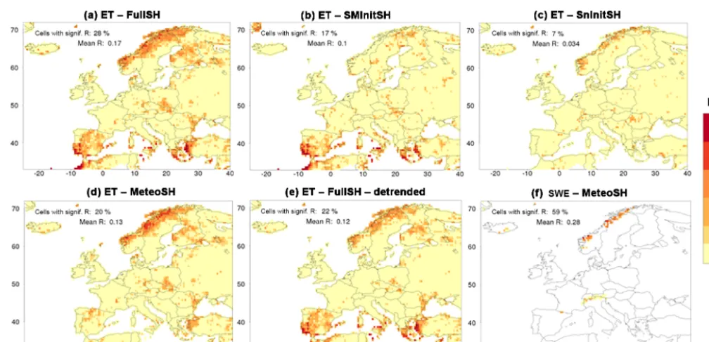
condi-teoSHs exhibit hardly any skill, while the SMInitSHs have considerable skill in the Mediterranean (Fig. 11b–d), it can be concluded that the skill in this region is due to soil mois-ture initial conditions. So, in this particular case, knowledge of soil moisture conditions on 1 February still yields skill in evapotranspiration in July. This skill in the Mediterranean is not affected by detrending (compare Fig. 11a and e), so it does not have a climate-change component.
The skill in Norway has a more complicated origin. The three specific hindcasts show that it is due to a mix of ini-tial snow conditions (Fig. 11c) and meteorological forcing (Fig. 11d). The effect of the initial snow conditions (on 1 February) can be understood with the help of the analy-sis of run-off skill in the SnInitSHs (Fig. 7), which led to the conclusion that run-off skill caused by snow initialisation occurs at the end of the melt season, which is July in much of Norway. Therefore, in this country and in July the tim-ing of the disappearance of snow cover varies from year to year. This then has a considerable effect on evapotranspira-tion, since bare soil has, compared to snow, higher surface temperatures and hence more evapotranspiration in summer. The contribution to skill by forcing (Fig. 11d) fades with, but is not removed by, detrending (not shown here), so it has a part that is related to climate change and a part that is unre-lated to climate change. The climate-change-reunre-lated skill due to forcing resides in the temperature hindcasts, which have significant skill in this region at all lead times (Fig. 2f). The non-climate-change-related skill in the MeteoSHs for July is likely an indirect effect of the skill in the forcing (especially precipitation) during the first lead month (February). This leads to skill in snow water that is equivalent towards the end of February, which fades but has not disappeared completely on 1 July (Fig. 11f) and then causes skill in evapotranspira-tion at the end of the melt season.
4 Discussion
4.1 Comparison of skill with previous studies
Figure 11.Explanation of the skill in the hindcasts of evapotranspiration (ET) for July by taking lead month 5 as an example. The panels map the skill in evapotranspiration of the FullSHs(a), SMInitSHs(b), SnInitSHs(c), MeteoSHs(d)and the FullSHs after detrending(e).
(f)depicts skill of the hindcasts of snow-water equivalent (SWE) in the MeteoSHs. For more explanation, see Fig. 1a. Note that statistics in the legends of the panels refer only to that part of the domain for whichRwas computed, which consists of all coloured cells.
consequence of forcing with inter-annual variation that has no or insufficient skill, such as the S4 forcing. Other stud-ies compared the FullSHs (also called climate-model-based hindcasts) with ESP hindcasts, which are slightly different from our InitSHs (see Sect. 4.3) but like the InitSHs have uninformative meteorological forcing for each year. Some of these studies (e.g. Singla et al., 2012; Mackay et al., 2015) found little overall difference in skill between the FullSHs and ESP hindcasts. However, in a study of Canadian catch-ments, Bazile et al. (2017) broadly confirm our finding that beyond the first lead month, ESP is superior to the FullSHs, while the reverse holds for the first lead month. Arnal et al. (2018) compared FullSHs with ESP hindcasts and found that, in Europe, ESP has more discrimination skill
[image:13.612.44.548.232.475.2]skill in the seasonal run-off forecasts produced with WUSHP. Contributions to skill by the initial conditions of snow and by the meteorological forcing are mostly much smaller. To our knowledge, two other studies analysed sources of skill of hy-drological seasonal forecasts for Europe with dynamical sys-tems similar to those of the present study, namely Bierkens and van Beek (2009) and Singla et al. (2012). Comparing our results with those of Bierkens and van Beek (2009), both studies agree that initial conditions form the dominant source of skill. However, compared to the present study, Bierkens and van Beek (2009) find a larger contribution to skill by the meteorological forcing, at least in summer. This differ-ence might be due to the quality of the forcing. Bierkens and van Beek (2009) developed an analogue events method to select, on the basis of annual sea surface temperature (SST) anomalies in the North Atlantic, annual ERA40 meteorolog-ical forcings, which they used as forcing for their hydrolog-ical model. One might speculate that in Europe their semi-statistical forcing is more skilful than the S4 forcing used in WUSHP. This suggests that there is room for improve-ment of climate-model seasonal forecasts, so if and when this improvement is realised, the relative contribution of the me-teorological forcing to skill in hydrological variables would increase. As for the second study of the sources of skill, con-clusions of Singla et al. (2012) are not directly comparable with those of the present study, as they used ESP and reverse ESP (see Sect. 4.3).
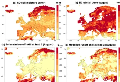
4.2 Understanding the skill due to initial soil moisture The dominance of soil moisture initial conditions in terms of domain-lumped skill also extends to the hotspot regions and periods of skill (Table 1). The understanding of the skill linked to soil moisture can be deepened by another level, as in Shukla and Lettenmaier (2011). The underlying idea is that this type of skill increases with the inter-annual variabil-ity of soil moisture at the date of initialisation and that this skill is gradually eliminated during the course of the hind-casts by inter-annual variability in processes like rainfall and snowmelt. The question is the following: to what extent are the hotspots of skill (see Table 1) linked to soil moisture ini-tialisation due to the cause of the skill, and to what extent they are due to a lack of inter-annual variability in the pro-cesses that eliminate the skill? Figure 12 helps answer this question for the skill found in the run-off hindcasts of August
σSM2
This estimate (Fig. 12c) needs to be compared with the skill of the hindcasts, mapped in Fig. 12d in terms ofR. The two maps are not expected to be exactly equal, not only because of the simplicity of the estimation method but also because Sestis not a correlation coefficient. However, in the limits, Sest has the desired properties. It is equal to zero for the
cases of constant initial amounts of soil moisture or infinite variability in rainfall. It is equal to 1 for the cases of infi-nite variability in soil moisture or constant rainfall. The cor-relation coefficient between the patterns in Fig. 12c and d is highly significant (0.67), and the hotspot regions of skill are the same in both panels, namely the northern part of Fennoscandia and the southern part of the Mediterranean. So, in the case of August as lead month 2 the estimation method is reasonably successful in computing the pattern of skill in the hindcasts with the simple means of the WFDEI data set and model calculations from the reference simulation. The merit of the estimation method is the deeper understanding of the cause of the skill in the two hotspot regions. North-ern Fennoscandia is a hotspot, because the amount of inter-annual variability in initial soil moisture is larger than else-where (Fig. 12a). The southern part of the Mediterranean is a hotspot, because the amount of inter-annual variability in rainfall is lower than elsewhere (Fig. 12b).
This simple method of analysis helped to bring the under-standing of the skill in northern Fennoscandia and the south-ern Mediterranean to a deeper level, but it was less successful for the other hotspots. A more thorough analysis along these lines and a deeper understanding of skill in the hindcasts is left for future work.
4.3 Relation of the present specific hindcasts with conventional ESP
The specific hindcasts of this study are related to the well-known ESP (e.g. Wood and Lettenmaier, 2008; Shukla and Lettenmaier, 2011; Singla et al., 2012; Van Dijk et al., 2013; Harrigan et al., 2018). ESP is not only used as an experimen-tal tool in science but is also widely used to produce forecasts in operational mode (Day, 1985). ESP used for scientific pur-poses can be subdivided into proper ESP (called ESP from now on) and reverse ESP.
Figure 12.Illustration of a simple method that partly explains skill in run-off due to initial soil moisture, exemplified for target month August as lead month 2.(a)is a map of the standard deviation in soil moisture at the date of initialisation (1 June). Similarly,(b)maps the standard deviation of observed rainfall during the course of the hindcasts (June–August). These two standard deviations are combined into an estimate of the skill (Eq. 1) in(c), which is compared with the skill of the FullSHs(d). Note that the colour scales of(c)and(d)differ from each other and differ from scales of other figures (e.g. Fig. 1a).
to year and are quasi-perfect, i.e. they are taken from a simu-lation like our reference simusimu-lation, while the meteorological forcing is uninformative, e.g. by being the same for all years (in the InitSHs and, for example, in the ESP of Shukla and Lettenmaier, 2011) or by varying randomly from year to year (e.g. in the ESP of Singla et al., 2012). This eliminates skill due to the meteorological forcing, so skill can only be due to the initial conditions. However, while in ESP the forcing is selected from historic observations, it is selected from the S4 hindcasts in InitSHs in order to retain an inter-member vari-ability and other statistical characteristics of the time series similar to that in the FullSHs. An advantage of ESP is that its production is relatively cheap, because no climate-model forecasts are needed.
Similarly, reverse ESP (see Wood and Lettenmaier, 2008) resemble the MeteoSHs of this study. In both types of hind-casts the meteorological forcing varies from year to year, while the initial conditions are identical for each year. This eliminates skill due to the initial conditions, so skill can only be due to the forcing. However, while in reverse ESP the forc-ing of each year is made up of the observations of that year, it is made up of the S4 hindcasts in the MeteoSHs. More-over, in reverse ESP, ensembles are built by using differing initial conditions, whereas they are built by using differing meteorological forcings in the MeteoSHs.
In ESP and in the InitSHs, if all skill due to the meteoro-logical forcing is indeed removed, the remaining skill, which is due to the annually varying initial conditions, should logi-cally be the same in both types of hindcasts, since the initial conditions are the same. To test this expectation we produced ESP and compared its skill with that of the InitSHs. Indeed, skill from these two types of hindcasts is almost identical, as demonstrated in the Supplement (Fig. S8). We conclude that skill produced with specific hindcasts with a forcing that does not vary from year to year is not sensitive to the choice of that forcing, perhaps with the exception of forcings that deviate strongly from being realistic. We like to note here that, in odd years, one of the ESP ensemble members is identical to the pseudo-observation used for verification. This is a concern, but we deemed this less important than the requirement of identical forcing for all years, which is crucial for the expla-nation of the skill reversal (Sect. 3.2.1).
We plan to launch an operational version of WUSHP. That version might include a post-processing procedure with the aims of removing biases in discharge and making the system more reliable. This could perhaps be done with statistical cal-ibration (e.g. Gneiting et al., 2005; Schepen et al., 2014), a technique that, contrary to quantile mapping, considers infor-mation that is available from correlations between hindcasts and observations (see Wood and Schaake, 2008; Madadgar et al., 2014).
The superiority of the InitSHs (and the ESP) with respect to the FullSHs for hindcasts beyond the first 2 lead months raises the question of whether one should, in an operational version of WUSHP and for these lead months, issue forecasts like the InitSHs (or ESP) and not forecasts like the FullSHs. The logical answer is “yes”, but such a strategy should then be reconsidered when the meteorological forcing is taken from a new, possibly improved version of the climate model or from another, possibly better type of climate model.
The applied methods of analysis are not suitable for giving quantitative advice on what would be the best investment for increasing the amount of skill of WUSHP. However, since initial soil moisture is the dominant source of predictability, a large gain of skill could possibly be made by assimilation of soil moisture observations into the modelled state of soil moisture (see e.g. Draper and Reichle, 2015). In addition, ob-servations of a snow-water equivalent could be assimilated into the modelled state of snow (see e.g. Griessinger et al., 2016). Improving the calibration of VIC would be another obvious road towards improvement of the seasonal predic-tions discussed in this paper. This should lead to higher ac-tual skill but not necessarily to more theoretical skill (see the discussion section of the companion paper).
5 Conclusions
The present paper explains skill in the hindcasts of WUSHP, a seasonal hydrological forecast system, applied to Europe. We first analysed the meteorological forcing, which con-sists of bias-corrected output from a climate model (S4), and found considerable skill in the precipitation forecasts of the first lead month but negligible skill for later lead times. Sea-sonal forecasts for temperature have more skill. Skill in sum-mer temperatures was found to be related to climate change occurring in both the observations and the hindcasts, and it
all years but with “perfect” initial conditions (InitSHs) pro-duce, averaged across the model domain, more skill in run-off than the hindcasts forced with S4 output (FullSHs). This occurs because inter-annual variability of the S4 forcing adds noise, while it has hardly any skill. The other specific hind-casts showed that in Europe initial conditions of soil mois-ture form the dominant source of skill in run-off. For target months from April to July, initial conditions of snow con-tribute significantly, with a domain-mean maximum in May and June. The timing of that maximum varies spatially and coincides with the end of the melt season, when snowmelt differs from year to year, because snow stops being available for melt at different dates. All regional and temporal hotspots of skill in run-off found in the companion paper are due to initial conditions of soil moisture, with smaller or larger con-tributions by the initial conditions of snow for target months from April to July in hotspot regions with snowfall in earlier months. We further showed that skill due to snow and soil moisture initialisation is more or less additive.
Some remarkable skill features are due to indirect effects, i.e. skill due to forcing or initial conditions of snow and/or soil moisture is, during the course of the model simulation, stored in the hydrological state (snow and/or soil moisture), which then by itself acts as a source of skill.
Predictability of evapotranspiration was analysed in some detail. Levels of predictability and the annual cycle of skill are similar to those for temperature. For most combinations of target and lead months, forcing forms the most important contributor to skill, but for lead month 2, initial conditions of soil moisture dominate from June to October.
– For each grid cell and combination of a category (or ter-cile; AN, NN and BN), lead month and target month we proceeded as follows:
– Divide the 30 (number of years) observations into terciles and give them a binary number (1 if the event falls in the considered category and otherwise 0).
– Divide the 450 (number of years×number of en-semble members) forecasts into terciles.
– Determine, for each of the 30 years, the forecast probability of the event occurring (forecast falling in the considered tercile).
– Pair the binary observations with the forecast prob-abilities.
– Sort the paired data into eight bins stratified by the forecast probabilities of the event.
– Compute bin averages of the forecast probability and of the binary observations.
– Pool the results for two consecutive lead months and the 3 target months of the same season.
– The results were further processed as follows:
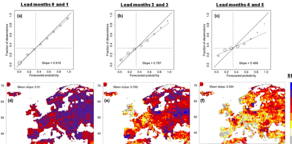
– They were aggregated for the entire domain and then plotted. Examples for the BN tercile and the spring months (MAM) as a target are shown in Fig. A1a–c, with the lead month number increas-ing from left to right. In each diagram a linear re-gression is applied to the data points, weighing in-dividual points by the number of data pairs in the bins. Because tercile thresholds are set indepen-dently for observations and forecasts, the resulting line always goes through the climatological inter-section (one-third in our case; see Weisheimer and Palmer, 2014), and results are insensitive to biases. As in Weisheimer and Palmer (2014) we use the slope of the line as a measure of reliability. A slope equal to 1 corresponds to perfect reliability, and a slope equal to 0 indicates no reliability at all.
denses to two points at the coordinates [0,0] and [1,1], which represent, respectively, two-thirds and one-third of all contributing data. In this case the hindcasts are utterly reli-able and utterly sharp. The second case is when the hindcasts have no discrimination skill at all, i.e. forecast probabilities of an event are randomly paired with the outcome (whether the event occurs or not). In this case, the slope of the fitted line is equal to zero, so the hindcasts are not reliable at all, and sharpness is minimal, i.e. forecast probabilities tend to approach one-third for each of the terciles.
In Fig. A1 reliability is evaluated for the case of verifica-tion with pseudo-observaverifica-tions. For the first 2 lead months, the slope of the line in the diagram of the aggregated data (Fig. A1a) is 0.916. Hence, during these 2 lead months the system is not far from being perfectly reliable, and it is rather sharp with relative maxima in forecast probability in the low-est and the highlow-est bin. Then, with progressing lead time, reliability is reduced, i.e. the slope of the aggregated data decreases to 0.767 (for lead months 2 and 3; Fig. A1b) and 0.469 (for lead months 4 and 5; Fig. A1c). Moreover, with in-creasing lead time, sharpness is reduced, with gradually more ensemble forecasts approaching the climatological forecast, i.e. a probability of one-third for each of the terciles.
The maps of Fig. A1d–f show the geographical distribu-tion of the slope from the reliability diagrams. For the first 2 lead months most values of the slope for individual grid cells lie between 0.7 and 1.1 (Fig. A1d), and the domain-averaged slope is 0.910. At longer leads, the highest val-ues are found in some regions with considerable amounts of discrimination skill, such as Poland and northern Germany, western France, and Romania and Bulgaria (see Table 1). Re-liability also tends to increase towards the northeast of the continent. Domain mean values of the grid-level slope are generally somewhat lower than the slope of the aggregated data. This can, at least partly, be ascribed to more scatter of individual points around the best-fit line because of the much smaller sample size for individual grid cells.
Figure A1.Reliability of the FullSH discharge hindcasts for the BN tercile in spring (target months MAM). Pseudo-observations were used for verification. Lead time increases from left to right. Aggregated reliability diagrams for the full domain are depicted in(a–c). The forecasted probabilities of BN discharge (horizontal axis) are collected in eight bins. The vertical co-ordinate is the relative frequency of BN discharge observations for all of the forecasts in a specific bin. The solid line is the 1:1 line. The dashed line shows the best fit to the eight data points, each weighted by the number of observations contributing to the bin (Nbin). The area of the symbols is proportional toNbin. The dotted lines are the averages of the variables along the two axes (one-third). Similar reliability diagrams were made for all grid cells individually, and the slopes of the best-fit lines are plotted in(d)–(f).
that for verification with real instead of pseudo-observations, slopes are closer to zero, so forecasts seem to be less reliable and more overconfident. Strikingly, discrimination skill and reliability have similar characteristics. Both decrease with in-creasing lead time, and differences between the AN and BN terciles are relatively small, while scores for the NN tercile are clearly inferior to those for the two outer terciles. Also, regional maxima in discrimination skill and reliability tend to coincide, and scores of discrimination skill and reliability are smallest in autumn.
Appendix B: Skill in the meteorological forcing before bias correction
Section 3.1 contains an analysis of the skill of the meteo-rological forcing after bias correction. Because predictabil-ity of the meteorological forcing is an interesting topic by itself, we present here an analysis of the skill of the mete-orological forcing before bias correction, i.e. of the raw S4 output, again limiting attention to the three variables consid-ered in Sect. 3.1. Figure B1a summarises the skill of the raw precipitation hindcasts, which should be compared with the summary for the bias-corrected hindcasts of precipitation in Fig. 1b. Such a comparison is made for lead months 0, 1 and 2 in Fig. B1b. Similar comparisons are made for the 2 m
Competing interests. The authors declare that they have no conflict of interest.
Special issue statement. This article is part of the special issue “Sub-seasonal to seasonal hydrological forecasting”. It is a result of the HEPEX workshop on seasonal hydrological forecasting in Norrköping, Sweden, on 21–23 September 2015.
Acknowledgements. This study was financially supported by the EUPORIAS project (EUropean Provision of Regional Impact Assessment on Seasonal-to-decadal timescale), grant agreement no. 308291, funded by the European Commission (EU) project in the Seventh Framework Programme. Revision of this paper was carried out in the research programme “JPI Climate & Belmont – Climate Predictability” under project number ALWCL.2016.1, funded by the Netherlands Organisation for Scientific Research (NWO).
Edited by: Ilias Pechlivanidis
Reviewed by: three anonymous referees
References
Arnal, L., Cloke, H. L., Stephens, E., Wetterhall, F., Prudhomme, C., Neumann, J., Krzeminski, B., and Pappenberger, F.: Skilful seasonal forecasts of streamflow over Europe?, Hydrol. Earth Syst. Sci., 22, 2057–2072, https://doi.org/10.5194/hess-22-2057-2018, 2018.
Baehr, J., Fröhlich, K., Botzet, M., Domeisen, D. I., Kornblueh, L., Notz, D., Piontek, R., Pohlmann, H., Tietsche, S., and Müller, W. A.: The prediction of surface temperature in the new sea-sonal prediction system based on the MPI-ESM coupled climate model, Clim. Dynam., 44, 2723–2735, 2015.
Bazile, R., Boucher, M.-A., Perreault, L., and Leconte, R.: Verifica-tion of ECMWF System 4 for seasonal hydrological forecasting in a northern climate, Hydrol. Earth Syst. Sci., 21, 5747–5762, https://doi.org/10.5194/hess-21-5747-2017, 2017.
Bierkens, M. F. P. and van Beek, L. P. H.: Seasonal predictability of European discharge: NAO and hydrological response time, J. Hydrometerol., 10, 953–968, 2009.
Crochemore, L., Ramos, M. H., Pappenberger, F., Andel, S. J. V., and Wood, A. W.: An experiment on risk-based decision-making
https://doi.org/10.5194/hess-19-4831-2015, 2015.
Ghile, Y. B. and Schulze, R. E.: Development of a framework for an integrated time-varying agrohydrological forecast system for Southern Africa: Initial results for seasonal forecasts, Water SA, 34, 315–322, 2008.
Gneiting, T., Raftery, A. E., Westveld III, A. H., and Goldman, T.: Calibrated probabilistic forecasting using ensemble model output statistics and minimum CRPS estimation, Mon. Weather Rev., 133, 1098–1118, 2005.
Greuell, W., Franssen, W. H. P., Biemans, H., and Hutjes, R. W. A.: Seasonal streamflow forecasts for Europe – Part I: Hindcast ver-ification with pseudo- and real observations, Hydrol. Earth Syst. Sci., 22, 3453–3472, https://doi.org/10.5194/hess-22-3453-2018, 2018.
Griessinger, N., Seibert, J., Magnusson, J., and Jonas, T.: Assess-ing the benefit of snow data assimilation for runoff modelAssess-ing in Alpine catchments, Hydrol. Earth Syst. Sci., 20, 3895–3905, https://doi.org/10.5194/hess-20-3895-2016, 2016.
Hagedorn, R., Doblas-Reyes, F. J., and Palmer, T. N.: The rationale behind the success of multi-model ensembles in seasonal fore-casting – I. Basic concept, Tellus A, 57, 219–233, 2005. Hamlet, A. F., Huppert, D., and Lettenmaier, D. P.: Economic
value of long-lead streamflow forecasts for Columbia River hy-dropower, J. Water Res. Plan. Man., 128, 91–101, 2002. Harrigan, S., Prudhomme, C., Parry, S., Smith, K., and
Tanguy, M.: Benchmarking ensemble streamflow prediction skill in the UK, Hydrol. Earth Syst. Sci., 22, 2023–2039, https://doi.org/10.5194/hess-22-2023-2018, 2018.
Kim, H. M., Webster, P. J., and Curry, J. A.: Seasonal prediction skill of ECMWF System 4 and NCEP CFSv2 retrospective fore-cast for the Northern Hemisphere Winter, Clim. Dynam., 39, 2957–2973, 2012.
Koster, R. D., Mahanama, S. P., Livneh, B., Lettenmaier, D. P., and Reichle, R. H.: Skill in streamflow forecasts derived from large-scale estimates of soil moisture and snow, Nat. Geosci., 3, 613– 616, 2010.
Li, H., Luo, L., and Wood, E. F.: Seasonal hydrologic predictions of low-flow conditions over eastern USA during the 2007 drought, Atmos. Sci. Lett., 9, 61–66, 2008.
Liang, X., Lettenmaier, D. P., Wood, E. F., and Burges, S. J.: A sim-ple hydrologically based model of land surface water and energy fluxes for general circulation models, J. Geophys. Res.-Atmos., 99, 14415–14428, 1994.
4) (p. 49), Reading, U. K: European Centre for Medium-Range Weather Forecasts, 2011.
Mushtaq, S., Chen, C., Hafeez, M., Maroulis, J., and Gabriel, H.: The economic value of improved agrometeorological informa-tion to irrigators amid climate variability, Int. J. Climatol., 32, 567–581, 2012.
Nijssen, B., O’Donnell, G. M., Lettenmaier, D. P., Lohmann, D., and Wood, E. F.: Predicting the discharge of global rivers, J. Cli-mate, 14, 3307–3323, 2001.
Richardson, D. S.: Measures of skill and value of ensemble predic-tion systems, their interrelapredic-tionship and the effect of ensemble size, Q. J. Roy. Meteor. Soc., 127, 2473–2489, 2001.
Scaife, A. A., Arribas, A., Blockley, E., Brookshaw, A., Clark, R. T., Dunstone, N., Eade, R., Fereday, D., Folland, C. K., Gor-don, M., and Hermanson, L.: Skillful long-range prediction of European and North American winters, Geophys. Res. Lett., 41, 2514–2519, 2014.
Schepen, A., Wang, Q. J., and Robertson, D. E.: Seasonal forecasts of Australian rainfall through calibration and bridging of coupled GCM outputs, Mon. Weather Rev., 142, 1758–1770, 2014. Shukla, S. and Lettenmaier, D. P.: Seasonal hydrologic
predic-tion in the United States: understanding the role of initial hy-drologic conditions and seasonal climate forecast skill, Hydrol. Earth Syst. Sci., 15, 3529–3538, https://doi.org/10.5194/hess-15-3529-2011, 2011.
Shuttleworth, J. S.: Evaporation, in: Handbook of Hydrology, 1992, edited by: Maidment, D. R., McGraw-Hill, New York, 1993. Singla, S., Céron, J.-P., Martin, E., Regimbeau, F., Déqué, M.,
Ha-bets, F., and Vidal, J.-P.: Predictability of soil moisture and river flows over France for the spring season, Hydrol. Earth Syst. Sci., 16, 201–216, https://doi.org/10.5194/hess-16-201-2012, 2012. Soares, M. B. and Dessai, S.: Barriers and enablers to the use of
seasonal climate forecasts amongst organisations in Europe, Cli-matic Change, 137, 89–103, 2016.
Sun, S., Jin, J., and Xue, Y.: A simple snow-atmosphere-soil transfer model. J. Geophys. Res.-Atmos., 104, 19587–19597, 1999.
climate service for water resource management, Adv. Sci. Res., 13, 51–55, 2016.
Weedon, G. P., Balsamo, G., Bellouin, N., Gomes, S., Best, M. J., and Viterbo, P.: The WFDEI meteorological forcing data set: WATCH Forcing Data methodology applied to ERA-Interim re-analysis data, Water Resour. Res., 50, 7505–7514, 2014. Weisheimer, A. and Palmer, T. N.: On the reliability of
sea-sonal climate forecasts, J. R. Soc. Interface, 11, 20131162, https://doi.org/10.1098/rsif.2013.1162, 2014.
Willmott, C. J., Rowe, C. M., and Mintz, Y.: Climatology of the terrestrial seasonal water cycle, J. Climatol., 5, 589–606, 1985. Wood, A. W. and Lettenmaier, D. P.: An ensemble approach for
attribution of hydrologic prediction uncertainty, Geophys. Res. Lett., 35, L14401, https://doi.org/10.1029/2008GL034648, 2008. Wood, A. W. and Schaake, J. C.: Correcting errors in streamflow forecast ensemble mean and spread, J. Hydrometerol., 9, 132– 148, 2008.
Wood, A. W., Kumar, A., and Lettenmaier, D. P.: A retrospec-tive assessment of National Centers for Environmental Predic-tion climate model–based ensemble hydrologic forecasting in the western United States, J. Geophys. Res.-Atmos., 110, D04105, https://doi.org/10.1029/2004JD004508, 2005.
Yuan, X., Wood, E. F., Luo, L., and Pan, M.: CFSv2-based seasonal hydroclimatic forecasts over the conterminous United States, J. Climate, 26, 4828–4847, 2013.
Yuan, X., Wood, E. F., and Ma, Z.: A review on climate-model-based seasonal hydrologic forecasting: physical understanding and system development, Wiley Interdisciplinary Reviews: Wa-ter, 2, 523–536, 2015.