A hybrid model of self organizing maps and least square support vector machine for river flow forecasting

(1)

Hydrol. Earth Syst. Sci., 16, 4417–4433, 2012 www.hydrol-earth-syst-sci.net/16/4417/2012/ doi:10.5194/hess-16-4417-2012

Hydrology and

Earth System

Sciences

A hybrid model of self organizing maps and least square support

vector machine for river flow forecasting

S. Ismail1, A. Shabri2, and R. Samsudin3

1_{Department of Mathematics, Science Faculty, Universiti Teknologi Malaysia, Malaysia} 2_{Department of Software Engineering, Faculty of Computer Science and Information System,}

Universiti Teknologi Malaysia, Malaysia

Correspondence to: S. Ismail ([email protected]), A. Shabri ([email protected])

Received: 18 May 2010 – Published in Hydrol. Earth Syst. Sci. Discuss.: 18 October 2010 Revised: 31 August 2012 – Accepted: 11 September 2012 – Published: 26 November 2012

Abstract. Successful river flow forecasting is a major goal

and an essential procedure that is necessary in water resource planning and management. There are many forecasting tech-niques used for river flow forecasting. This study proposed a hybrid model based on a combination of two methods: Self Organizing Map (SOM) and Least Squares Support Vector Machine (LSSVM) model, referred to as the SOM-LSSVM model for river flow forecasting. The hybrid model uses the SOM algorithm to cluster the entire dataset into several dis-jointed clusters, where the monthly river flows data with similar input pattern are grouped together from a high di-mensional input space onto a low didi-mensional output layer. By doing this, the data with similar input patterns will be mapped to neighbouring neurons in the SOM’s output layer. After the dataset has been decomposed into several disjointed clusters, an individual LSSVM is applied to forecast the river flow. The feasibility of this proposed model is evaluated with respect to the actual river flow data from the Bernam River located in Selangor, Malaysia. The performance of the SOM-LSSVM was compared with other single models such as ARIMA, ANN and LSSVM. The performance of these models was then evaluated using various performance indi-cators. The experimental results show that the SOM-LSSVM model outperforms the other models and performs better than ANN, LSSVM as well as ARIMA for river flow forecasting. It also indicates that the proposed model can forecast more precisely, and provides a promising alternative technique for river flow forecasting.

1 Introduction

Hydrological data such as flows and rainfall are the basic information used in the design of water resource systems. Knowledge about the characteristics and volume of river flow is very important, especially for predicting the future river flow in the monsoon season where the heavy rainfall may cause heavy river flow, potentially causing problems such as flooding and erosion. Reduced river flow is likely to restrict the supply of water for domestic use and industrial and hy-droelectric power generation. Therefore, the ability to fore-cast future river flow would be beneficial in the field of water management and help in the design of flood protection works in urban areas and for agricultural land.

In hydrology, different types of models are used such as lumped conceptual models, physically-based models, also known as knowledge-driven modelling, and empirical mod-els, also known as data-driven modelling. By using knowl-edge driven modelling, the other catchment variables such as catchment characteristics (size, shape, slope and storage characteristics of the catchment), and geomorphologic char-acteristics of a catchment (topography, land use patterns, vegetation and soil types that affect the infiltration) must be considered because it is hypothesized that forecasts could be improved if catchment characteristic variables which affect flow were to be included (Jain and Kumar, 2007; Dibike and Solomatine, 2001).

River flow forecast can be generated using two types of mathematical models: rainfall-runoff models and river flow models. The rainfall-runoff models use both climatic and hydrologic data, while river flow models only use the

(2)

4418 S. Ismail et al.: River flow forecasting

hydrologic data. The river flow process in a catchment area is a complex process that can be affected by many inter re-lated physical factors. The factors affecting the river flow response of a catchment subjected to rainfall input include storm characteristics, such as intensity and duration of rain-fall events, and so on. Moreover, the conceptual rainrain-fall- rainfall-runoff models need a large amount of data for calibration and validation purposes and are usually computationally expen-sive and very time consuming (Grayson et al., 1992; Jain and Kumar, 2007). Although combining other variables may im-prove their prediction accuracy, but in practice, especially in developing countries like Malaysia, such information is often either not available or difficult to obtain. Moreover, the influ-ence of these variables and many of their combinations in generating river flow is an extremely complex physical pro-cess, especially due to the data collection of multiple inputs and parameters, which vary in space and time and which are not clearly understood (Zhang and Govindaraju, 2000; Jain and Kumar, 2007).

Owing to the complexity of this process, many researchers are focusing on river flow forecasting, which only consid-ers the past river flow data, because it offconsid-ers a rapid devel-opment and minimum information requirement (Adamowski and Sun, 2010; Kisi, 2004, 2008; Wang et al., 2009). This data-driven modelling by using historical data which are based on extracting and re-using the information that is im-plicitly contained in the hydrological data without taking directly into account any physical load that underlies the rainfall-runoff process provides accurate and rapid develop-ment time with minimum data information.

River flow forecasting is an important yet difficult task in the field of hydrology because predicting future events in-volves a decision-making process where the ability to pre-dict future river flow will provide the right edge and assist the engineers in terms of flood control management, and pro-vide some benefits in the areas of water supply management (Viessman et al., 1989). Accurate continuous data collections on the catchment area are needed to produce a good river flow forecast. There are many forecasting techniques that have been proposed in the literature for river flow forecasting. The most comprehensive of all popular and widely-known statis-tical methods used in time series forecasting is the Autore-gressive Integrated Moving Average (ARIMA) model, also known as the Box Jenkins model. Several studies have shown that ARIMA can be trusted as a reliable model in water re-sources time series analysis (Muhamad and Hassan, 2005; Huang et al., 2004; Modarres, 2007; Fernandez and Vega, 2009; Wang et al., 2009) ).

Among the non-linear approaches, the Artificial Neural Network (ANN) is the most widely used for time series fore-casting and has been successfully employed in the modelling of a wide range of hydrologic contexts (Maier and Dandy, 2000; Dibike and Solomatine, 2001; Bowden et al., 2005; Dolling and Varas, 2003; Muhamad and Hassan, 2005; Kisi, 2008; Wang et al., 2009; Keskin and Taylan, 2009; Luk et

al., 2000; Hung et al., 2009; Affandi and Watanabe, 2007; Birkinshaw et al., 2008; Corzo et al., 2009). ANN provides an attractive alternative tool for forecasting and has shown its nonlinear modelling capabilities in data time series forecast-ing. However, the selection of an optimal network structure (layers and nodes) and training algorithms always needs the attention of modellers (Maier and Dandy, 2000). The net-work structure is usually determined by using a trial-and-error approach (Kisi, 2004).

Recently, the support vector machine (SVM) method, which was suggested by Vapnik (1995), has been used in hy-drological modelling such as stream flow forecasting (Asefa, et al., 2006), flood stage forecasting (Yu et al., 2006), rain-fall runoff modelling (Dibike et al., 2001; Elshorbagy et al., 2010a, b), etc. However, the standard SVM is based on the structural risk minimal principal and involves complicated quadratic programming methods, which are often time con-suming and have a higher computational burden because of the required constrained optimization programming.

As a simplification of SVM, Suykens et al. (2002) pro-posed the use of the least squares support vector machines (LSSVM). LSSVM has been used successfully in various areas of pattern recognition and regression problems (Han-bay, 2009; Kang et al., 2008). LSSVM encompasses simi-lar advantages to SVM, but its additional advantage is that it only requires the solving of a set of linear equations, which is much easier and computationally simpler. The method uses equality constraints instead of inequality constraints and adopts the least squares linear system as its loss function, which is computationally attractive. LSSVM also has good convergence and high precision. Hence, this method is eas-ier to use than quadratic programming solvers in the SVM method. Extensive empirical studies (Wang and Hu, 2005) have shown that LSSVM is comparable to SVM in terms of general performance. In the area of water resources, the LSSVM method has received very little attention in the liter-ature and there are only a few applications of LSSVM in the modelling of environmental and ecological systems such as water quality prediction (Yunrong and Liangzhong, 2009).

(3)

S. Ismail et al.: River flow forecasting 4419

2004). However, SOM has been successfully utilized as a first step in clustering algorithms.

The Self Organizing Map (SOM), proposed by Koho-nen (2001), is one category of ANN that was first used as an information-processing tool in the fields of speech and im-age recognition. SOM has been successfully applied in clus-tering, classification, estimation, prediction and data min-ing (Vesanto and Alhoniemi, 2000; Kohonen, 2001). SOM can be used as a clustering tool since it converts the non linear statistical relationship between high dimensional data into simple geometric relationships of their image points on a low-dimensional display. From that, the data points which show similar properties are placed close to each other within the output of the SOM algorithm (Budayan et al., 2009). After the SOM training is finished, one can figure out the number of clusters directly by eye according to the two-dimensional map (Lin and Chen, 2005). Clustering the dataset may seem unnecessary; however, it is an important task especially when dividing a complex problem into sev-eral smaller and simpler problems can more easily be solved compared with the original problem (Jacobs et al., 1991; Lin and Chen, 2006; Lin and Wu, 2007; Wu and Chau, 2009; Wu et al, 2009).

SOM has attracted increasing interest for water resources application, such as the classification of satellite imagery data and rainfall estimation (Murao et al., 1993), rainfall-rounoff modelling (Hsu et al., 2002), typhoon-rainfall fore-casting (Lin and Wu, 2009), river flood forefore-casting (Chang et al., 2007), water resource problems (Kalteh et al., 2008), and model evaluation (Herbst and Casper, 2008; Herbst et al., 2009). The advantages of SOM compared with the other clustering methods have been extensively discussed in the literature (Chen et al., 1995; Mangiameli et al., 1996; Lin and Chen, 2006). Mangiameli et al. (1996) showed that the SOM performed the best when compared to seven other hi-erarchical clustering methods. Lin and Chen (2006) recom-mend SOM as an alternative to the identification of homo-geneous regions for regional frequency analysis where the results showed that the SOM determines the cluster member-ship more accurately than the K-means method and Ward’s method. In addition, the SOM is more robust than the tra-ditional clustering methods. Lin and Chen (2005) apply the SOM clustering for predicting the groundwater head at Hsiu-Lin Station, Taiwan. Among 240 datasets, the first 192 sam-ples are used for training and the remaining 48 samsam-ples are used for testing. The entire datasets are then mapped into 14×14 map sizes. The map is then divided into 15 regions or clusters to continue with the prediction model using RBFN.

Improving forecasting accuracy, especially in time series forecasting, is an important yet often difficult task facing decision-makers in many areas. Using hybrid models has become common practice to improve forecasting accuracy. There are several studies that show that hybrid models can be an effective way to improved the accuracy of forecasting, compared to using single models separately (Zhang, 2003;

Jain and Kumar, 2007; Chen and Wang, 2007; Pai and Lin, 2005; Hsu et al., 2009). For instance, Lin and Wu (2009) proposed a combination of SOM and MLP in order to fore-cast the typhoon rainfall at Tanshui River Basin. SOM was used to analyze and divide the input data into distinct clus-ters. The second step involved an individual relationship be-tween the input and output data constructed by a specific MLP. For evaluating the forecasting performance of the pro-posed model, an application was conducted. The results show that the proposed model can forecast more precisely than the model developed by the conventional neural network ap-proach. Srinivas et al. (2009) combined a SOM and fuzzy clustering for regional flood frequency analysis for water-sheds data from Indiana, USA. Results show that the pro-posed approach performs better in estimating flood quantiles at ungauged sites.

In recent years more hybrid models have been proposed, which combine a clustering technique with local forecast-ing models that are more accurate since these models are more specialised and have successfully solved many predic-tions problems, such as a combination of SOM with ANN (Pal et al., 2003; Lin and Wu, 2009; Wang and Yan, 2004), SOM with SVM (Cao, 2003; Fan and Chen, 2006; Fan et al., 2007; Huang and Tsai, 2009), SOM with Radial Basis Function (Lin and Chen, 2005), ANN with K-means (Corzo and Solomantine, 2007) and other models (Chang and Liao, 2006; Chang et al., 2007, 2008). Although the idea of these hybrid models is interesting and promising, it still need to be tested using a river flow time series.

Based on the same idea by Tay and Cao (2001) and Hsu et al. (2009), this study aims to explore the application of hybrid technique and to test the capability and effectiveness of the idea of hybrid modelling which combines the SOM with the LSSVM (LSSVM). The hybrid model SOM-LSSVM is then proposed for river flow forecasting in order to improve the accuracy of prediction. With the advantages of the data analysis technique developed by SOM and the capa-bility of LSSVM, the proposed hybrid model is expected to be useful for river flow forecasting. The results of the predic-tions by the SOM-LSSVM model are compared with a fore-casting model developed by conventional ARIMA, ANN and LSSVM models. To verify the application of this approach, the monthly river flow for Bernam River located in Selangor, Malaysia was analyzed as a case study in this research.

2 Data-driven modelling

Data-driven modelling is considered as a tool in building a model that will replace the knowledge-driven modelling in describing a physical behaviour (Solomatine et al., 2008). However, the data-driven models may not correctly represent the input–output mapping if the modelled system changed during the time when the data are collected. Therefore, it is necessary for the entire dataset to go through a statistical

(4)

analysis test to prove whether there are some other trends in the dataset. Trend analysis on time series data has been proven to be a useful tool for effective water resources plan-ning, design, and management (Douglas et al., 2000; Hamil-ton et al., 2001), since trend detection of hydrological vari-ables such as river flow provide useful information on the possibility of change tendency of the variables in the future (Yue and Wang, 2004).

Another issue that still remains a question is the num-ber of the appropriate data that can be used to predict fu-ture river flows by using data-driven modelling. Number of data also plays an important role in predicting future river flows. For example, Kisi and Cimen (2010) used the monthly river flow data of Canakdere River and Goksudere River in their research. The observed data are 40 yr (480 months) along with an observation period between 1960 and 1999 for both stations. Jain and Kumar (2007) applied their proposed model using monthly river flow data for a period of 62 yr (1911–1972) derived from the Colorado River at Lees Ferry, CO, USA, for modelling a hydrologic time series forecast-ing. Usually, the monthly data are used to estimate the wa-ter demand and the wawa-ter supply (Srikanthan and McMahon, 2001). Although river flow forecasting models using histor-ical river flow time series data may lack the ability to vide physical interpretation and insight into catchment pro-cesses, they are nevertheless able to provide relatively accu-rate flow forecasts and become more and more popular in hydrological modelling due to their rapid development times and minimum information requirements.

3 Forecasting models

This section presents the ARIMA, ANN, LSSVM and SOM-LSSVM models used for river flow forecasting. The choice of these models in this study was due to the fact that these methods have been widely and successfully used in time series forecasting.

3.1 The Autoregressive Integrated Moving Average

Model

The Box-Jenkins model, also know as Autoregressive Inte-grated Moving Average (ARIMA), was introduced by Box and Jenkins (1970) and has been one of the most popular ap-proaches in the area of forecasting. The order of an ARIMA model is represented by ARIMA (p,d,q)and the order of the seasonal ARIMA or SARIMA model is represented by ARIMA (p,d,q)×(P,D,Q)s, where the term (p,d,q)is

the order of the non-seasonal and (P,D,Q)s is the order of

the seasonal. The general ARIMA models are a compound of a seasonal and non-seasonal part and are represented in the following manner:

φp(B)8P(Bs)(1−B)d(1−Bs)Dxt=θq(B)2Q(Bs)at, (1)

whereφ (B)andθ (B)are polynomials of orderpandq, re-spectively;8(Bs)and2(Bs)are polynomials inBs of de-greesP andQ, respectively;pis the order of non-seasonal auto regression;dis the number of regular differencing;qis the order of the non-seasonal moving average;P is the or-der of seasonal autoregression;Dis the number of seasonal differencing;Qis the order of seasonal moving average;B is the backward shift operator, andsis the length of the sea-son. Random errorsat are assumed to be independently and identically distributed with a mean of zero and a constant variance ofσ2.

The ARIMA model involves four steps, which are the identification step, estimation step, diagnostic checking step and forecasting step. In the identification step, the sample au-tocorrelation function (ACF) and sample partial autocorrela-tion funcautocorrela-tion (PACF) are used to determine whether or not the series is stationary and if it is seasonal or non-seasonal. If the series is not stationary, then a transformation called differencing is needed until the series reaches the stationary level. ACF as well as PACF are used to choose a tentative model. Once a tentative model is identified, the parameters of the model are estimated. Diagnostic checking using the ACF and PACF of the residuals is carried out, basically to check whether the model’s assumptions about the errorat are sat-isfied. If the model is not adequate, a new tentative model should be identified followed by the steps of parameter esti-mation and model verification. The process is repeated sev-eral times until finally a satisfactory model is selected. The forecasting model is then used to compute the fitted values and forecasts values.

3.2 Artificial neural network

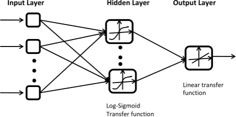
The ANN is flexible computing, which has been extensively studied and used for time series forecasting in many areas of science and engineering since early 1990. The most com-monly used ANN in the field of water resources and hydrol-ogy is the feed forward multi layer perceptron (MLP), which consists of three layers: the first is the input layer where the data are introduced to the network, the second layer is the hidden layer where the data are processed, and the final layer is the output layer where the results of the given in-put are produced. The structure of a feed-forward ANN is shown in Fig. 1.

Mathematically, a three-layer MLP withpinput nodes,q hidden nodes and one output node can be expressed as

yt =g q X j=1

wjf p X i=1

wixt−i !!

, (2)

(5)

37

1 Fig 1. The Architecture Of Three Layers Feed-Forward Back-Propagation ANN

2

3

4

5

6 Fig 2. The SOM architecture

7

8

9

10

11

12

13

Linear transfer function

Log-Sigmoid Transfer function

[image:5.595.49.285.64.181.2]

Input Layer Hidden Layer Output Layer

Fig. 1. The architecture Of three layers feed-forward

backpropaga-tion ANN.

f (.)as the linear function are adopted here. The equations for linear function and sigmoid function are as follows:

Linear: f (x)= purelin(x)=xi (3)

,

Log-Sigmoid: f (x)= logsig(x)= 1

1+exp(−x). (4) Training a network is an essential factor for the success of neural networks. Among the several learning algorithms available, backpropagation has been the most popular and most widely implemented learning algorithm for all neural network paradigms (Zou et al., 2007). In a backpropagation network, the weighted connections only feed activations in the forward direction from an input layer to the output layer. These interconnections are adjusted using an error conver-gence technique where the best match for the network’s re-sponse is the desired rere-sponse. Backpropagation is the most popular algorithm for training feed-forward MLP. For de-tailed reviews of ANN, along with their application in water resources and hydrology, the reader can be referred to Maier and Dandy (2000).

3.3 Least Squares Support Vector Machine

The Least Squares Support Vector Machine (LSSVM) is a modification of the standard Support Vector Machine (SVM), and was developed by Suykens and Vandewalle (Suykens, 2002). The basic LSSVM is used for the opti-mal control of non-linear Karush-Kuhn-Tucker systems for classification as well as regression. The LSSVM predictor is trained using a set of time series historic values as inputs and a single output as the target value. In the following, we briefly introduce LSSVM and its use in time series forecasting.

Consider a set of dataD={(x1,y1), (x2,y2),...,(xn,yn)}, xi∈ <p,yi ∈ <,xis the input vector,yis the expected output andn is the number of data. The LSSVM approximate the function in the following form:

y(x)=wTϕ(x)+b, (5)

whereφ (x)represents the high dimensional feature spaces, which is non-linearly mapped from the input space x. By

combining the functional complexity and fitting error, the op-timization problem of LSSVM is given as

min:

J (w, ξ )=1 2w

T_w₊γ 2

n X

i=1

ξ;2

i (6)

subject to:

y(x)=wTϕ(xi)+b+ξii=1,2,3, ..., n. (7) This formulation consists of equality instead of inequality constraints. To solve this optimization problem, the Lagrange function is constructed as

L(w, b, ξ;α)=J (w, b, ξ )

− n X

i=1

αi{wTϕ(xi)+b−yi+ξi}, (8)

whereαi are the Lagrange multipliers, which can be posi-tive or negaposi-tive. The solution of Eq. (8) can be obtained by partially differentiating with respect tow, b, ξi andαi 

               

∂L

∂w =0→w= n P i=1

αiϕ(xi)

∂L ∂b =0→

n P i=1

αi=0 ∂L

∂ξi =0→αi=γ ξi

∂L

∂αi =0→w

T_ϕ(x

i)+b−yi+ξi=0

fori=1,2,3, ...n.

(9) After elimination of the variableswandξi, one obtains the following matrix solution:

0 1T

1φ (xi)Tφ (xl)+γ−1I b α

=

0 y

, (10)

with y= [y1, y2, ..., yl], 1Tv = [1,1, ...,1],α= [α1, α2, ...,

αl]. The kernel function can be defined as

K(xi, xj)=φ (xi)Tφ (xj), i, j=1,2, ..., n. (11) This finally leads to the following LSSVM model for regression:

y(x)= n X i=1

αiK(xi, xj)+b, (12)

where αi, b are the solutions to the linear system and K(xi, xj)is a kernel function. The most popular kernel func-tion is the Radial Basis Funcfunc-tion (RBF), as shown in Eq. (13) (Liu and Wang, 2008; Gencoglu and Ulyar, 2009).

K(xi, xj)=exp −

kx−xik2 δ2

!

. (13)

(6)

37

1 Fig 1.

The Architecture Of Three Layers Feed-Forward Back-Propagation ANN

2

3

4

5

6 Fig 2.

The SOM architecture

7

8

9

10

11

12

13

Linear transfer function

Log-Sigmoid Transfer function

Input Layer Hidden Layer Output Layer

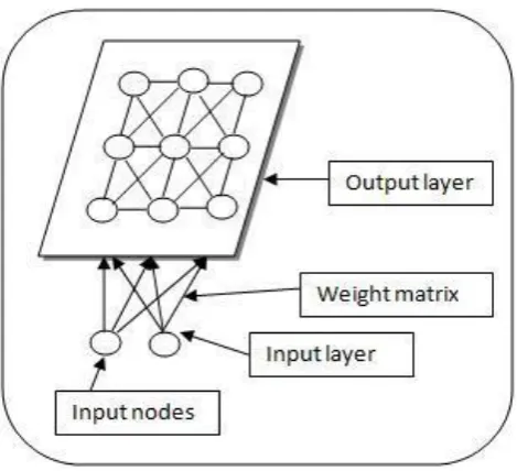
Fig. 2. The SOM architecture.

3.4 Self organizing map

SOM, also known as the Self Organizing Feature Map (SOFM), was proposed by Professor Teuvo Kohonen and therefore sometimes called the Kohonen Map (Kohonen, 2001), is an unsupervised and competitive learning algo-rithm. SOM has been used widely for data analysis in some areas such as economics, physics, chemistry as well as medical applications.

The objectives of SOM are to maximize the degree of sim-ilarity of patterns within a cluster, minimize the simsim-ilarity of patterns belonging to different clusters, and then present the results in a lower-dimensional space. Basically, SOM con-sists of two layers of artificial neurons: the input layer, which accepts the external input signals; and the output layer, also called the output map, which is usually arranged in a two-dimensional structure. Every input neuron is connected to ev-ery output neuron, and each connection has a weighting value attached to it. The architecture of SOM is shown in Fig. 2.

Output neurons will self organize to an ordered map, and neurons with similar weights are placed together. They are connected to adjacent neurons by a neighbourhood relation, dictating the topology of the map (Moreno et al., 2006). The concept of the learning algorithm for SOM is unsupervised and competitive. The training process of SOM is described below:

For simplicity, we assume that the input vector X of SOM is:

X= [x1, x2, ..., xn], (14)

wherenis the dimension of the input vector. The weight vec-tor connecting the input vecvec-tor to the hidden neuroniis de-noted by

Wi= [wi1, wi2, ..., win] i=1,2, ..., m. (15) The weights are initialised as small random numbers at the start of the training process. In competitive learning net-works, the neurons compete among themselves to determine the winner by calculating the distance between the input vec-tor and the weight vecvec-tors of all the neurons in the hidden layer. The winnerIis defined as the one whose weight vector is the closet to the input vectorX:

I (X)=min ∀i

kX−Wik i=1,2, ..., m. (16) The Euclidean distance is often used as the similarity mea-sure for SOM. The output neuron whose weight vector has the smallest distance from the input vector is called the winning neuron.

After determining the winning neuron, the lateral inter-sections between the winning neuron and its neighbourhood are calculated using the topological neighbourhood function. The neighbourhood function takes the form of a radial ba-sis function that is appropriate for representing the biological lateral interaction (Kohonen, 2001; Rui Xu, 2009):

hj i(t )=η(t )exp

−||rj−ri||2 2σ2_{(t )}

!

, (17)

where||rj−ri||represents the Euclidean distance between the winning neuron i and the neighbouring neuronj, and σ (t )is the bandwidth of the radial basis kernel function.

Next, the weights of this winning neuron are adjusted ac-cording to the input patterns using the algorithm

Wi(t+1)=Wi(t )+hj i(t )(X−Wi(t )), (18) whereη(t )is the learning rate at timet andWi(t+1)is the adjusted weight vector at time(t+1).

After the weights have been updated, the winning neu-ron and the neighbourhood neuneu-rons become more simi-lar to the corresponding input pattern. The process contin-ues until convergence has been reached. Finally, the trained SOM is obtained.

3.5 Integrating the SOM-LSSVM model

[image:6.595.50.285.60.274.2]

(7)

38 1

2 3

Fig 3. The SOM-LSSVM architecture 4

5

6

7

8

Fig 4. The Study Area 9

10

Fig. 3. The SOM-LSSVM architecture.

38 1

2 3

Fig 3. The SOM-LSSVM architecture 4

5

6

7

8

Fig 4. The Study Area 9

10

Fig. 4. The study area.

data points with similar statistical distribution are grouped to-gether. Each group or cluster contains similar objects (Huang and Tsai, 2009). After the clustering of the data into several groups, LSSVMs are constructed for each cluster. LSSVM can conduct a better forecast for each group or cluster. As demonstrated by Tay and Cao (2001) and Hsu et al. (2009), this hybrid model can capture better results in the prediction of future river flow.

4 The study area and data

In this research, we examined the data obtained from the monthly river flow of the Bernam River located in Selan-gor, Penisular Malaysia. Bernam River is located between the states of Perak and Selangor, demarcating the border be-tween the two states. The upper Bernam River basin has been identified as the ultimate and largest source of water supply from the Bernam River, especially for irrigation and the sup-ply of drinking water. The study area is about 1090 km2with a mean elevation of 19 m, and the Bernam River monitoring station is the downstream outlet. The location of the Bernam River catchment is shown in Fig. 4.

The monthly river flow data of the Bernam River, con-sisting of 516 monthly records (January 1966 to December 2008), are used in this study. The data were first tested using Mann-Kendall test in order to detect any other trends in river flow data. After that, the dataset was then split up into two

39 1

Fig 5. Time Series of Monthly River Flow of Bernam River (Jan. 1966-Dis.2008) 2

3

4

5

6

7

8

9

10

11

12

13

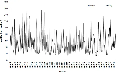
Fig. 5. Time series of monthly river flow of Bernam River

(Jan-uary 1966–Dezember 2008).

parts: training and testing, where the first dataset consisting of 456 monthly records (January 1966 to December 2003) was used for training, while the final dataset containing 60 mean monthly river flows (January 2004 to December 2008) was used for testing. Training data were used exclusively for model development and testing data were used to mea-sure the performance of the model on untrained data. The testing set was also used to evaluate the forecasting ability of the model and to compare the proposed model with oth-ers. The recorded time series data for the Bernam River are shown in Fig. 5.

Solomatine et al. (2008) suggested that when splitting data into training and testing datasets, these sets should have sim-ilar distributions of low and high flow or simsim-ilar properties of the input and output variables. However, it has been found that to generalise the training and testing sets with similar properties is not an easy task. Most studies suggest that the ratio of splitting for training and testing should be [70:30, 80:20, or 90:10]. The selection of the ratio could be based on the particular problem under consideration (Zhang et al., 1998; Firat, 2007; Kisi, 2008; Wang et al., 2009). Before the training process begins, data normalisation is often per-formed. The river flow was normalised in the range [0.1, 0.9] by the following equation:

yt =0.1+ xt 1.2(xmax)

, (19)

whereytrepresents the normalised data, whilextis the actual observation value and xmax represents the maximum value

among the actual observation values.

5 Input determination

As with any data-driven model such as ANN and LSSVM, the selection of appropriate model inputs plays an extremely important role in their successful implementation since it provides the basic information about the system being mod-elled. In time series forecasting, usually insufficient attention

[image:7.595.49.285.60.187.2] [image:7.595.311.547.62.208.2]

(8)

[image:8.595.117.476.81.194.2]

Table 1. Model of input data.

Model Input Data

M1 yt=f (xt−1, xt−2)

M2 yt=f (xt−1, xt−2, xt−3, xt−4)

M3 yt=f (xt−1, xt−2, xt−3, xt−4, xt−5, xt−6)

M4 yt=f (xt−1, xt−2, xt−3, xt−4, xt−5, xt−6, xt−7, xt−8)

M5 yt=f (xt−1, xt−2, xt−3, xt−4, xt−5, xt−6, xt−7, xt−8, xt−9, xt−10)

M6 yt=f (xt−1, xt−2, xt−3, xt−4, xt−5, xt−6, xt−7, xt−8, xt−9, xt−10, xt−11, xt−12)

M7 yt=f (xt−1, xt−2, xt−4, xt−5, xt−7, xt−10, xt−12)(Stepwise)

M8 yt=f (xt−1, xt−2, xt−12, xt−13, xt−14, xt−24, xt−25, xt−26, at−12, at−24)(ARIMA)

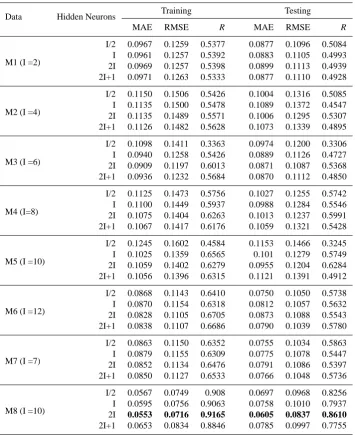
Table 2. The result for the training and testing using ANN model.

Data Hidden Neurons Training Testing

MAE RMSE R MAE RMSE R

M1 (I =2)

I/2 0.0967 0.1259 0.5377 0.0877 0.1096 0.5084 I 0.0961 0.1257 0.5392 0.0883 0.1105 0.4993 2I 0.0969 0.1257 0.5398 0.0899 0.1113 0.4939 2I+1 0.0971 0.1263 0.5333 0.0877 0.1110 0.4928

M2 (I =4)

I/2 0.1150 0.1506 0.5426 0.1004 0.1316 0.5085 I 0.1135 0.1500 0.5478 0.1089 0.1372 0.4547 2I 0.1135 0.1489 0.5571 0.1006 0.1295 0.5307 2I+1 0.1126 0.1482 0.5628 0.1073 0.1339 0.4895

M3 (I =6)

I/2 0.1098 0.1411 0.3363 0.0974 0.1200 0.3306 I 0.0940 0.1258 0.5426 0.0889 0.1126 0.4727 2I 0.0909 0.1197 0.6013 0.0871 0.1087 0.5368 2I+1 0.0936 0.1232 0.5684 0.0870 0.1112 0.4850

M4 (I=8)

I/2 0.1125 0.1473 0.5756 0.1027 0.1255 0.5742 I 0.1100 0.1449 0.5937 0.0988 0.1284 0.5546 2I 0.1075 0.1404 0.6263 0.1013 0.1237 0.5991 2I+1 0.1067 0.1417 0.6176 0.1059 0.1321 0.5428

M5 (I =10)

I/2 0.1245 0.1602 0.4584 0.1153 0.1466 0.3245 I 0.1025 0.1359 0.6565 0.101 0.1279 0.5749 2I 0.1059 0.1402 0.6279 0.0955 0.1204 0.6284 2I+1 0.1056 0.1396 0.6315 0.1121 0.1391 0.4912

M6 (I =12)

I/2 0.0868 0.1143 0.6410 0.0750 0.1050 0.5738 I 0.0870 0.1154 0.6318 0.0812 0.1057 0.5632 2I 0.0828 0.1105 0.6705 0.0873 0.1088 0.5543 2I+1 0.0838 0.1107 0.6686 0.0790 0.1039 0.5780

M7 (I =7)

I/2 0.0863 0.1150 0.6352 0.0755 0.1034 0.5863 I 0.0879 0.1155 0.6309 0.0775 0.1078 0.5447 2I 0.0852 0.1134 0.6476 0.0791 0.1086 0.5397 2I+1 0.0850 0.1127 0.6533 0.0766 0.1048 0.5736

M8 (I =10)

I/2 0.0567 0.0749 0.908 0.0697 0.0968 0.8256 I 0.0595 0.0756 0.9063 0.0758 0.1010 0.7937 2I 0.0553 0.0716 0.9165 0.0605 0.0837 0.8610

2I+1 0.0653 0.0834 0.8846 0.0785 0.0997 0.7755

[image:8.595.121.477.242.678.2]

(9)

40

Lag P a rt ia l A u to c o rr e la ti o n 65 60 55 50 45 40 35 30 25 20 15 10 5 1 1.0 0.8 0.6 0.4 0.2 0.0 -0.2 -0.4 -0.6 -0.8 -1.0

Partial Autocorrelation Function for Sg Bernam

(with 5% significance limits for the partial autocorrelations)

Lag A u to c o rr e la ti o n 65 60 55 50 45 40 35 30 25 20 15 10 5 1 1.0 0.8 0.6 0.4 0.2 0.0 -0.2 -0.4 -0.6 -0.8 -1.0

Autocorrelation Function for Sg Bernam

(with 5% significance limits for the autocorrelations)

1 Fig 6.

ACF and PACF For Monthly River Flow of Bernam River

2

3

4

5

6

66 60 54 48 42 36 30 24 18 12 6 1 1.0 0.8 0.6 0.4 0.2 0.0 -0.2 -0.4 -0.6 -0.8 -1.0 Lag A u to co rr e la ti o n

ACF of Residuals for Sg Bernam

66 60 54 48 42 36 30 24 18 12 6 1 1.0 0.8 0.6 0.4 0.2 0.0 -0.2 -0.4 -0.6 -0.8 -1.0 Lag P a rt ia l A u to co rr e la ti o n

PACF of Residuals for Sg Bernam

7 Fig 7.

The ACF And PACF of Residuals For Monthly River Flow Of Bernam River for

8 ARIMA (2, 0, 0) x (2, 0, 2)

12

model

9

10

11

12

40

1 Fig 6.

ACF and PACF For Monthly River Flow of Bernam River

2

3

4

5

6

7 Fig 7.

The ACF And PACF of Residuals For Monthly River Flow Of Bernam River for

8 ARIMA (2, 0, 0) x (2, 0, 2)

12

model

9

10

11

12

Fig. 6. ACF and PACF for monthly river flow of Bernam River.

is given to the task of selecting appropriate model inputs. Many papers reviewed failed to describe the input determi-nation methodology used, and consequently raised doubts about the optimality of the output obtained (Bowden et al., 2005). Most researchers design experiments to help select the model inputs, while others adopt some empirical ideas. For example, Patil (1992) proposed model inputs based on 12 inputs for monthly data and four for quarterly data heuris-tically. Cheung et al. (1996) suggested maximum entropy principles to identify the time series lag structure. Tang and Fishwick claimed that the number of model inputs is sim-ply the number of the autoregressive (AR) moving average components in the Box-Jenkins models. Refenes et al. (2003) suggested a stepwise method for determining the input for ANN models. Roadknight et al. (1997) used cross correla-tion analysis or principal component analysis as a guide for determining the input. Aqil et al. (2006) employed two sta-tistical methods, i.e. autocorrelation (ACF) and partial au-tocorrelation (PACF), to identify the appropriate input vari-ables. Behzad et al. (2009) selected the best model inputs by trial and error according to minimum test errors in the ANN

40

1 Fig 6.

ACF and PACF For Monthly River Flow of Bernam River

2

3

4

5

6

7 Fig 7.

The ACF And PACF of Residuals For Monthly River Flow Of Bernam River for

8 ARIMA (2, 0, 0) x (2, 0, 2)

12

model

9

10

11

12

40

1 Fig 6.

ACF and PACF For Monthly River Flow of Bernam River

2

3

4

5

6

7 Fig 7.

The ACF And PACF of Residuals For Monthly River Flow Of Bernam River for

8 ARIMA (2, 0, 0) x (2, 0, 2)

12

model

9

10

11

12

Fig. 7. The ACF And PACF of residuals for monthly river flow of

Bernam River for ARIMA (2, 0, 0) x (2, 0, 2)12model.

and SVM modelling. Corzo et al. (2009) used correlation and average mutual information analysis involving different sub-basin values using precipitation and river flow to determine the best input variables. Khashei and Bijari (2010) proposed an ARIMA model to determine the input variables in order to yield a more accurate forecasting model than ANN. The em-pirical results from three well-known real datasets showed that the proposed input variables can be an effective way to improve the forecasting accuracy achieved by ANN. The use of input variables from the data values of previous time se-ries and the optimum number of input variables determined by trial and error has been reported by Firat (2007, 2008), Firat and Gungor (2007), Sivapragasam and Liong (2005), Juhos et al. (2008), Partal and Kisi (2007), among others.

Three approaches were used in this study to deter-mine the models of input data. The first six approaches for the input data were chosen based on past river flow. The appropriate lags were chosen using a trial-and-error approach (xt−1, xt−2,. . . , xt−p, where p is 2, 4, . . . , 12). It gives the number of inputs (I) as 2, 4, 6, 8, 10, 12. The second and third approaches set the input vector nodes equal to the number of lagged variables from two statistical methods (i.e. stepwise multiple regression

(10)

[image:10.595.50.286.81.203.2]

Table 3. The result for the training and testing using LSSVM model.

Data Training Testing MAE RMSE R MAE RMSE R

M1 0.0955 0.1248 0.5494 0.0858 0.1080 0.5191 M2 0.0850 0.1120 0.6757 0.0860 0.1084 0.5207 M3 0.0829 0.1120 0.6647 0.0797 0.1000 0.6092 M4 0.0853 0.1134 0.6564 0.0812 0.1021 0.6037 M5 0.0773 0.1035 0.7767 0.0800 0.1084 0.5232 M6 0.0744 0.1018 0.7308 0.0744 0.0995 0.6191 M7 0.0720 0.0970 0.7598 0.0771 0.1019 0.6756

M8 0.0486 0.0633 0.9259 0.0457 0.0611 0.8769

analysis and the ARIMA model). Stepwise multiple re-gression analysis led to the selection of 7 input attributes (xt−1, xt−2, xt−4, xt−5, xt−7, xt−10, xt−12).

In ARIMA, the future value of a variable is assumed to be a linear function of several past observations and random errors (Zhang, 2003; Khashei and Bijari, 2010). In this study, ARIMA (2, 0, 0)×(2, 0, 2)12 is selected as the best model,

as described in Sect. 6.1. Therefore, the functional form of the model input data using ARIMA is

yt=f (xt−1, xt−2, xt−12, xt−13, xt−14, xt−24, xt−25,

xt−26, at−12, at−24)

, (20)

whereyt is the future value,xt is the past value at timet and at is the residual at timet, where ARIMA is used in order to generate the residuals.

6 Evaluation of performance

There are different types of performance evaluation that have been documented in the literature (Luchetta and Manetti, 2003; Goswami et al., 2005). The performance evaluation for each model should have at least a measure of absolute error, such as mean absolute error (MAE) or root mean square er-ror (RMSE) (Legates and McCabe, 1999). Wang et al. (2006) stated that RMSE is a good performance evaluation mea-surement because it is very sensitive to even small errors, in which case it is better to compare the small differences in the model’s performance.

The MAE and RMSE are defined as follows: MAE =1_n

n P t=1

yt− ˆot

(20)

RMSE= v u u t 1 n

n X

t=1

yt− ˆot 2

(21)

whereyt and oˆt are the observed/actual and the predicted at the timet. The criteria to judge the best model are rela-tively small for MAE and RMSE in modelling and forecast-ing. Other than these, the correlation coefficient (R) was also used as a performance measurement.Rwas also used to test

the ability of the model to capture the complex nature of the process that was being modelled (Jain and Kumar, 2007; Lin and Wu, 2009). It is a measure of how well the future out-comes are likely to be predicted by the model, where the pre-dicted flows correlate with the observed flows.Ris defined as

R=

1

n n P t=1

(yt− ¯y)

ˆ

ot− ¯ˆo

s

1

n n P t=1

(yt− ¯y)2 s

1

n n P t=1

ot− ¯ˆo

2

, (22)

wherey¯ ando¯ˆ are the mean observed and mean predicted river flow series, respectively, and nis the number of data points. TheRvalue is used to evaluate the linear correlation between the observed and the predicted flow. Clearly, anR value close to unity indicates a satisfactory result, while a low value or one close to zero implies an inadequate result.

7 Experiment and results

[image:10.595.308.468.142.201.2]

7.1 Application of the ARIMA model

Figure 5 shows the plots of the river flow time series, indicat-ing that the time series are non-stationary and require a trans-formation. Samples of the autocorrelation function (ACF) and the partial autocorrelation function (PACF) for the se-ries are plotted in Fig. 6. The ACFs curves for the monthly stream flow data decayed with mixture of sine wave pattern and exponential curves, which reflect the random periodicity of the data and indicate the need for seasonal MA terms in the model. In the PACF there were significant spikes present near lag 12 and 24, therefore indicating the series need for a seasonal AR process. The criteria used to judge the best model based on MSE show that ARIMA (2, 0, 0)×(2, 0, 2)12is the best model. The model can be written as

(1−0.352B−0.132B2)(1−0.603B12−0.395B24) xt=(1−0.477B12−0.460B24)at, (23) and can be rewritten as

xt =0.352xt−1+0.132xt−2+0.603xt−12−0.212xt−13

+0.079xt−14+0.395xt−24−0.136xt−25−0.052xt−26

−0.477at−12−0.460at−24+at. (24) The ACF and PACF plots of the residuals of ARIMA (2, 0, 0)×(2, 0, 2)12for the river flow series are shown in Fig. 7.

From the residual plot of the best ARIMA model, it was ob-served that the selected ARIMA (2, 0, 0)×(2, 0, 2)12model

passed the diagnostic checks and they were all white noise. For further analysis, we decided that the ARIMA model (2, 0, 0)×(2, 0, 2)12 is the best to use for comparison with

(11)

[image:11.595.148.447.81.518.2]

Table 4. The result for the training and testing using a hybrid model of SOM-LSSVM for different map sizes.

Map Sizes Data Training Testing

MAE RMSE R MAE RMSE R

M1 0.0680 0.0903 0.7964 0.0740 0.0872 0.7508 M2 0.0655 0.0860 0.8205 0.0767 0.0963 0.6574 M3 0.0758 0.1031 0.7259 0.0785 0.1020 0.6072 2 x 2 M4 0.0686 0.0931 0.7925 0.0752 0.0975 0.6456 M5 0.0770 0.1045 0.7250 0.0784 0.0988 0.6322 M6 0.0869 0.1135 0.6495 0.0794 0.1022 0.5931 M7 0.0758 0.1051 0.7126 0.0764 0.1011 0.6082

M8 0.0212 0.0333 0.9782 0.0441 0.0620 0.8766

M1 0.0747 0.0997 0.7445 0.0640 0.0860 0.7376 M2 0.0532 0.0681 0.8908 0.0683 0.0879 0.7254 3 x 3 M3 0.0760 0.1029 0.7271 0.0736 0.0917 0.7099 M4 0.0736 0.0995 0.7517 0.0733 0.0908 0.7019 M5 0.0721 0.1008 0.7504 0.0734 0.0951 0.6650 M6 0.0685 0.0914 0.8049 0.0794 0.1067 0.5421 M7 0.0735 0.0974 0.7599 0.0703 0.0971 0.6474

M8 0.0278 0.0378 0.9705 0.0431 0.0622 0.8734

M1 0.0537 0.0751 0.8640 0.0557 0.0691 0.8457 M2 0.0561 0.0756 0.8642 0.0727 0.0884 0.7299 M3 0.0649 0.0885 0.8105 0.0741 0.0937 0.6841 4 x 4 M4 0.0696 0.0921 0.7947 0.0800 0.1010 0.6159 M5 0.0647 0.0920 0.7990 0.0686 0.0916 0.7005 M6 0.0645 0.0879 0.8253 0.0737 0.0992 0.6247 M7 0.0701 0.0933 0.7830 0.0620 0.0894 0.7117

M8 0.0348 0.0507 0.9485 0.0435 0.0647 0.8651

M1 0.0659 0.0950 0.7715 0.0637 0.0876 0.7274 M2 0.0446 0.0612 0.9127 0.0668 0.0838 0.7560 M3 0.0646 0.0920 0.7911 0.0690 0.0865 0.7361 5 x 5 M4 0.0550 0.0762 0.8762 0.0680 0.0870 0.7306 M5 0.0555 0.0782 0.8646 0.0727 0.0931 0.6855 M6 0.0385 0.0605 0.9231 0.0661 0.0850 0.7462 M7 0.0761 0.0982 0.7848 0.0731 0.0969 0.6490

M8 0.0401 0.0567 0.9299 0.0370 0.0492 0.9222

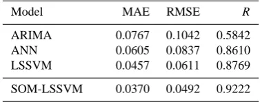
Table 5. Comparative performance between ARIMA, ANN,

LSSVM and SOM-LSSVM during the testing period.

Model MAE RMSE R

ARIMA 0.0767 0.1042 0.5842 ANN 0.0605 0.0837 0.8610 LSSVM 0.0457 0.0611 0.8769

SOM-LSSVM 0.0370 0.0492 0.9222

7.2 Application of ANN model

In this study, a typical three layer ANN model with a log-sigmoid transfer function from the input layer to the hidden

layer, and a linear function from the hidden layer to an out-put layer, are used for forecasting monthly river flow time se-ries. The input and target data were normalised in the range [0.1, 0.9], because a sigmoid function was employed as the transfer function. The network was trained for 5000 epochs using the conjugate gradient descent backpropagation algo-rithm with a learning rate of 0.001 and a momentum coeffi-cient of 0.9. The eight models of input data (M1–M8) with various numbers of input structures are trained and tested by ANN models, and the optimal number of neuron in the hid-den layer was ihid-dentified using several guidelines.

To help avoid the problem of over-fitting, some researchers have provided empirical rules to restrict the number of hidden nodes. In order to select an appropriate architec-ture, the following guidelines were used: “I/2” proposed by

[image:11.595.72.261.571.645.2]

(12)

Kang (1991), “I” proposed by Tang and Fishwick (1993), “2I” proposed by Wong (1991), and “2I+ 1” proposed by Hecht-Nielsen (1990), whereI is the number of inputs.

It is common to use one test set for both validation and testing purposes, particularly with small datasets (Zhang, 2003). For ANN experiment, the dataset was split into two sections: training set and test set where the test set was used for validation and testing purposes, as demonstrated by Zhang (2003) and Kisi (2004). The networks that yielded the best results with the lowest MAE and RMSE and largest R from the testing set were selected as the best ANN for the corresponding series. The effects of changing the num-ber of hidden nodes on the RMSE, MAE andR are shown in Table 2.

Table 2 shows the performance of ANN varying with the number of nodes in the hidden layer. For the training and test-ing period, the M8 model with 20 hidden nodes obtained the best results for MAE, RMSE andR, with statistics of 0.0553, 0.0716 and 0.9163, respectively. While in the testing phase, the M8 model with 20 hidden neurons was the best MAE, RMSE andR with statistics of 0.0606, 0.0837 and 0.8610, respectively. Hence, the ANN (10, 20, 1) has been selected as the most appropriate ANN model for the Bernam River.

7.3 Application of the LSSVM model

There is no single proven theory that can be used to guide the selection of the number of inputs. In this study, the same in-put structures of the datasets M1 to M8 were used. The RBF was used as the kernel function for this study. In order to bet-ter evaluate the performance of the proposed approach, we considered a grid search of(γ , σ2)withinnthe range 10 to 1000, andσ2in the range 0.01 to 1.0. For each hyper param-eter pair(γ , σ2)in the search space, 5-fold cross validation on the training set was performed to predict the prediction error. Table 3 shows the performance results obtained in the training and testing period of the LSSVM approach.

By considering these training and testing periods, the lowest MAE and RMSE and the largest R for the series of data were calculated from the M8 model, resulting in statistics of 0.0486, 0.0633, 0.9259 and 0.0457, 0.0611, 0.8769, respectively.

7.4 Application of the hybrid SOM-LSSVM model

Determining the appropriate map sizes of clustering is very important for cluster validity and efficiency. For a SOM of large map sizes, input patterns will be grouped into a large number of clusters, which would cause each neuron to memorise one of the input patterns, although some clus-ters may only have one or two members. Such clustering results are not suitable for the forecasting analysis. On the other hand, if the map size is too small, then many differ-ent data groups might be lumped into the same category and the SOM will fail to show the topological relationships of

the input patterns. Since there is no systematic or standard method for finding the optimal number of map sizes in the clustering algorithms, the optimal map size is obtained de-pending on the requirements of the user. In this paper, four map sizes are utilized, Kohonen of 2×2, 3×3, 4×4 and 5×5. When SOM is applied to perform cluster analysis, a SOM of a small dimension is the first choice. If the cluster-ing result is reasonable and satisfactory, then the cluster anal-ysis is accepted. Otherwise, a SOM of a larger dimension is chosen to analyse the input patterns, and this continues until a satisfactory result is obtained. In this study, only 4 clusters were considered to investigate the impacts of the number of map sizes on the performance. The same parameters were used as for the LSSVM’s parameters for the single LSSVM model. Table 4 shows the predicted values of SOM-LSSVM for the various numbers of map sizes.

7.5 Comparison

In this section, the predictive capabilities of the proposed SOM-LSSVM model are compared with ARIMA, ANN and LSSVM for the Bernam monthly river flow. Furthermore, the MAE, RMSE, andRare used to evaluate the performance of the ARIMA, ANN, LSSVM and SOM-LSSVM models. The statistical results of the different models are summarised in Table 5. From Table 5, it can be noted that the SOM-LSSVM model has the best performance with the lowest MAE and RMSE, and the largestR for the testing phase. The single LSSVM is the second best model, followed by ANN. As can be seen in Tables 5, ARIMA has the worst performance based on MAE, RMSE andR.

In the testing phase, the SOM-LSSVM model improved the ARIMA model with about a 52.78 % and 51.76 % re-duction in RMSE and MAE values, respectively, and with a 57.86 % improvement of the forecast results for theRvalue. SOM-LSSVM also produced some improvement over the ANN model with about a 45.16 % and 38.84 % reduction in RMSE and MAE, respectively, and some improvement in the forecast value of about 7.1 % forR. As with LSSVM, the SOM-LSSVM model resulted in some improvement over LSSVM as well, with about a 19.47 % reduction in RMSE, 19.03 % reduction in MAE and improvement of 5.16 % in the Rvalue.

(13)

41

1

2 Fig 8.

Predicted And Observed River Flow During Testing Period By ARIMA, ANN,

3 LSSVM And SOM-LSSVM For Bernam River

4

5

6

7

8

9

10

11

12

41

1

2 Fig 8.

Predicted And Observed River Flow During Testing Period By ARIMA, ANN,

3 LSSVM And SOM-LSSVM For Bernam River

4

5

6

7

8

9

10

11

12

41

1

2 Fig 8.

Predicted And Observed River Flow During Testing Period By ARIMA, ANN,

3 LSSVM And SOM-LSSVM For Bernam River

4

5

6

7

8

9

10

11

12

41

1

2 Fig 8.

Predicted And Observed River Flow During Testing Period By ARIMA, ANN,

3 LSSVM And SOM-LSSVM For Bernam River

4

5

6

7

8

9

10

11

12

Fig. 8. Predicted and observed river flow during testing period by

ARIMA, ANN, LSSVM and SOM-LSSVM for Bernam River.

42

1

2

Fig 9. The Scatter Plot Of Predicted And Observed River Flow During Testing Period Using

3

ARIMA, ANN, LSSVM And SOM-LSSVM For Bernam River 4

5

6

7

8

9

10

11

12

42

1

2

3

5

6

7

8

9

10

11

12

42

1

2 Fig 9.

The Scatter Plot Of Predicted And Observed River Flow During Testing Period Using

3 ARIMA, ANN, LSSVM And SOM-LSSVM For Bernam River

4

5

6

7

8

9

10

11

12

42

1

2

3

5

6

7

8

9

10

11

12

Fig. 9. The scatter plot of predicted and observed river flow during

testing period using ARIMA, ANN, LSSVM and SOM-LSSVM for Bernam River.

(14)

equation coefficients of the SOM-LSSVM are superior com-pared to the other models. The results indicate that the best performance can be obtained by the SOM-LSSVM model, followed by the LSSVM, ANN and ARIMA models. SOM-LSSVM can also give a better prediction performance than ARIMA, ANN and LSSVM time series approaches. The re-sults obtained in this study indicate that the SOM-LSSVM model is a powerful tool, as well as an alternative method for modelling river flow time series.

8 Conclusions

To improve the performance of river flow forecasting, a hy-brid model based on a combination of SOM and LSSVM was proposed to predict monthly river flows. Before apply-ing these models, the selections of the input data variables were conducted to determine the capability and suitability of the models to predict river flows. By using an evaluation on the performance test, the input data variables based on the ARIMA model were chosen as the optimal input factors. Next, SOM clustering technique was used to analyze these input data variables. The SOM algorithm clustered the entire input data into several disjointed clusters and after decom-posing the data, LSSVM was used to predict the river flow. The result shows that the performance of river flow fore-casting can be significantly enhanced by using the proposed hybrid SOM-LSSVM model.

To illustrate the capability of the SOM-LSSVM model, monthly river flow data from Bernam River were analyze in this study. The river flow data were varied per the number of input data used in the experiments. The number of input data variables were determine using the three approaches of past observation, stepwise regression analysis and ARIMA model. The experimental results show that SOM-LSSVM performs better than other models such as ARIMA, ANN and LSSVM. Through the comparison of four different mod-els applied in monthly river flow forecasting, it can be con-cluded that SOM-LSSVM provides a promising alternative technique for river flow time series forecasting. It can also be concluded that the selections of input data variables also play an important role in the prediction as well as the num-ber of Kohonen map sizes. In this study, only river flows data are considered for analysis, so future research can further test the idea of the hybrid model by employing the rainfall-runoff data, and using other clustering techniques such as K-Means or Fuzzy C-Means. Since this is an exploratory analysis of the hybrid SOM-LSSVM, the model should be further tested with another type of data with a variety of sample sizes to test the feasibility and ability of the SOM-LSSVM model. The idea of the hybrid model can also be tested on other time series data such as rainfall forecast, weather forecast, economic and so on to prove its capability and usability.

Acknowledgements. This research is supported by Zamalah

Schol-arship, Universiti Teknologi Malaysia and in part of E-Science, Ministry of Science, Technology and Innovation (MOSTI) funda-mental research grant scheme under vote number 79346.

Edited by: D. Solomatine

References

Adamowski, J. and Sun, K.: Development of a coupled wavelet transform and neural network method for flow forecasting of non-perennial rivers in semi-arid watersheds, J. Hydrol., 390, 85–91, 2010.

Affandi, A. K. and Watanabe, K.: Daily groundwater level fluctu-ation forecasting using soft computing technique, Nat. Sci., 5, 1–10, 2007.

Aqil, M., Kita, K., and Macalino, M.: A Preliminary study on the suitability of data driven approach for continuous water laeve modeling, Int. J. Comp. Sci., 1, 246–252, 2006.

Asefa, T., Kemblowski, M., McKee, M., and Khalil, A.: Multi-time scale stream flow predictions: The support vector machines ap-proach, J. Hydrol., 318, 7–16, 2006.

Behzad, M., Asghari, K., Eazi, M., and Palhang, M.: Generalization performance of support vector machines and neural networks in runoff modeling, Expert Syst. Appl., 36, 7624–7629, 2009. Birkinshaw, S. J., Parkin, G., and Rao. Z.: A hybrid neural networks

and numerical models approach for predicting groundwater ab-straction impacts, J. Hydroinform., 10, 127–137, 2008. Box, G. E. P. and Jenkins, G.: Time Series Analysis, Forecasting

and Control, Holden-Day, San Francisco, CA, 1970.

Budayan, C., Dikmen, I., and Birgonul, M. T.: Comparing the per-formance of traditional cluster analysis, self-organizing maps and fuzzy C-means method for strategic grouping, Expert Syst. Appl., 36, 11772–11781, 2009.

Bowden, G. J., Dandy, G. C., and Maier, H. R.: Input determination for neural network models in water resources application. Part 1-background and methodology, J. Hydrology, 301, 75–92, 2005. Cao, L.: Support vector machines experts for time series

forecast-ing, Neurocomputforecast-ing, 51, 321–339, 2003.

Chang, F. J., Chang, L. C., and Wang, Y. S.: Enforced self-organizing map neural networks for river flood forecasting, Hy-drol. Process., 21, 741–749, 2007.

Chang, P. C. and Liao, T. W.: Combining SOM and fuzzy rule base for flow time prediction in semiconductor manufacturing factory, Appl. Soft Comput., 6, 198–206, 2006.

Chang, P. C., Fan, C. Y., and Wang, Y. W.: Evolving CBR and data segmentation by SOM for flow time prediction in semiconductor manufacturing factory, J. Intell. Manuf., 20, 421–429, 2008. Chen, K. Y. and Wang, C. H.: A hybrid SARIMA and support

vec-tor machines in forecasting the production values of machinery industry in Taiwan, Expert System Application, 32, 254–264, 2007.

(15)

Cheung, K. H., Szeto, K. Y., and Tam, K. Y.: Maximum-entropy ap-proach to identify time-series lag structure for developing intelli-gent forecasting systems, International Journal of Computational Intellegence and Organization, 1, 94–106, 1996.

Corzo, G. A. and Solomantine, D. P.: Baseflow separation tech-niques for modular artificial neural network modelling in flow forecasting, Hydrolog. Sci. J., 52, 491–507, 2007.

Corzo, G. A., Solomatine, D. P., Hidayat, de Wit, M., Werner, M., Uhlenbrook, S., and Price, R. K.: Combining semi-distributed process-based and data-driven models in flow simulation: a case study of the Meuse river basin, Hydrol. Earth Syst. Sci., 13, 1619–1634, doi:10.5194/hess-13-1619-2009, 2009.

Douglas, E. M., Vogel, R. M., and Kroll, C. N.: Trends in floods and low flows in the United States: impact of spatial correlation, J. Hydrol., 240, 90–105, 2000.

Dibike, Y. B., Velickov, S., Solomatine, D. P., and Abbott, M. B.: Model induction with support vector machines: introduction and applications, ASCE J. Comput. Civil Eng., 15, 208–216, 2001. Dibike, Y. D. and Solomatine, D. P.: River flow forecasting using

artificial neural networks, Phys. Chem. Earth (B), 26, 1–7, 2001. Dolling, O. R. and Varas, E. A.: Artificial neural networks for

streamflow prediction, J. Hydraul. Res., 40, 547–554, 2003. Elshorbagy, A., Corzo, G., Srinivasulu, S., and Solomatine, D.

P.: Experimental investigation of the predictive capabilities of data driven modeling techniques in hydrology – Part 1: Con-cepts and methodology, Hydrol. Earth Syst. Sci., 14, 1931–1941, doi:10.5194/hess-14-1931-2010, 2010a.

Elshorbagy, A., Corzo, G., Srinivasulu, S., and Solomatine, D. P.: Experimental investigation of the predictive capabilities of data driven modeling techniques in hydrology – Part 2: Application, Hydrol. Earth Syst. Sci., 14, 1943–1961, doi:10.5194/hess-14-1943-2010, 2010b.

Fan, S. and Chen, L.: Short-term load forecasting based on an adap-tive hybrid method, IEEE Transactions on Power System, 21, 392–401, 2006.

Fan, S., Mao, C., and Chen, L.: Next-day electricity-price forecast-ing usforecast-ing a hybrid network. IET. Gener. Transm. Distrib. 1, 176– 182, 2007.

Fernandez, C. and Vega, J. A.: Streamflow drought time series fore-casting: a case study in a small watershed in north west spain, Stoch. Environ. Res. Risk Assess., 23, 1063–1070, 2009. Firat, M.: Comparison of Artificial Intelligence Techniques for

river flow forecasting, Hydrol. Earth Syst. Sci., 12, 123–139, doi:10.5194/hess-12-123-2008, 2008.

Firat, M. and Gungor, M.: Hydrological time-series modeling using an adaptive neuro-fuzzy inference system, Hydrol. Process., 18, 833–844, 2007.

Gencoglu, M. T. and Uyar, M.: Prediction of flashover voltage of in-sulators using least square support vector machines, Expert Sys-tems with Applications, 36, 10789–10798, 2009.

Grayson, R. B., Moore, I. D., and McMahon, T. A.: Physically based hydrologic modelling. 2. Is the concept realistic, Water Resour. Res., 28, 2659–2666, 1992.

Goswami, M., O’Connor, K. M., Bhattarai, K. P., and Shamseldin, A. Y.: Assessing the performance of eight real-time updating models and procedures for the Brosna River, Hydrol. Earth Syst. Sci., 9, 394–411, doi:10.5194/hess-9-394-2005, 2005.

Hamilton, J. P., Whitelaw, G. S., and Fenech, A.: Mean annual tem-perature and annual precipitation trends at Canadian biosphere reserves, Envir. Monit. Assess, 67, 239–275, 2001.

Hanbay, D.: An expert system based on least square support vector machines for diagnosis of valvular heart disease, Expert Systems with Applictions, 36, 8368–8374, 2009.

Hecht-Nielsen, R.: Neurocomputing, Menlo Park, CA., Addison-Wesley, 1990

Herbst, M. and Casper, M. C.: Towards model evaluation and iden-tification using Self-Organizing Maps, Hydrol. Earth Syst. Sci., 12, 657–667, doi:10.5194/hess-12-657-2008, 2008.

Herbst, M., Gupta, H. V., and Casper, M. C.: Mapping model be-haviour using Self-Organizing Maps, Hydrol. Earth Syst. Sci., 13, 395–409, doi:10.5194/hess-13-395-2009, 2009.

Hsu, K., Gupta, H. V., Gao, X. Sorooshian, S., and Imam, B.: Self-organizing linear output map (SOLO): an artificial neural net-work suitable for hydrologic modeling and analysis, Water Re-sour. Res., 38, 1302, doi:10.1029/2001WR000795, 2002. Hsu, S.-H., Hsieh, J. J. P.-A., Chih, T.-C., and Hsu, K.-C.: A

two-stage architecture for stock price forecasting by integrating self-organizing map and support vector regression, Expert Systems with Applications, 36, 7947–7951, 2009.

Huang, C. L. and Tsai, C. Y.: A hybrid SOFM-SVR with a filter-based feature selection for stock market forecasting, Expert Syst. Appl., 36, 1529–1539, 2009.

Huang, W., Bing Xu, B., and Hilton, A.: Forecasting flow in apalachicola river using neural networks, Hydrol. Process., 18, 2545–2564, 2004.

Hung, N. Q., Babel, M. S., Weesakul, S., and Tripathi, N. K.: An artificial neural network model for rainfall forecasting in Bangkok, Thailand, Hydrol. Earth Syst. Sci., 13, 1413–1425, doi:10.5194/hess-13-1413-2009, 2009.

Jain, A. and Kumar, A. M.: Hybrid neural network models for hy-drologic time series forecasting, Appl. Soft Comput, 7, 585–592, 2007.

Jacobs, R. A., Jordon, M. A., Nowlan, S. J., and Hinton, G. E.: Adaptive mixtures of local expert, Neural Compt., 3, 79–87, 1991.

Juhos, I., Makra, L., and Toth, B.: Forecasting of traffic orgin NO and NO2concentrations by Support Vector Machines and neural

networks using principal component analysis, Simulation Mod-eling Practice and Theory, 16, 1488–1502, 2008.

Kang, S.: An investigation of the Use of Feedforward Neural Net-work for Forecasting, Kent State University, Ph.D. Thesis, 1991. Kang, Y. W., Li, J., Cao, G. Y., Tu, H. Y., Li, J., and Yang, J.: Dy-namic temperature modeling of an SOFC using least square sup-port vector machines, J. Power Sources, 179, 683–692, 2008. Kalteh, A. M., Hjorth, P., and Berndtsson, R.: Review of the

self-organizing map (SOM) approach in water resources: Analysis, modeliong and application. Environ. Model. Softw., 23, 835– 845, 2008.

Khashei, M. and Bijari, M.: An artificial neural network (p,d,q) model for time series forecasting, Expert Syst. Appl., 37, 479– 489, 2010.

Keskin, M. E. and Taylan, D.: Artifical models for interbasin flow prediction in southern Turkey, 14, 752–758, 2009.

Kisi, O.: River flow modeling using artificial neural networks, J. Hydrol. Eng., 9, 60–63, 2004.