www.hydrol-earth-syst-sci.net/17/4323/2013/ doi:10.5194/hess-17-4323-2013
© Author(s) 2013. CC Attribution 3.0 License.
Hydrology and
Earth System
Sciences
On the importance of observational data properties when assessing
regional climate model performance of extreme precipitation
M. A. Sunyer1, H. J. D. Sørup1,2, O. B. Christensen2, H. Madsen3, D. Rosbjerg1, P. S. Mikkelsen1, and
K. Arnbjerg-Nielsen1
1Department of Environmental Engineering, Technical University of Denmark, Lyngby, Denmark 2Danish Climate Centre, Danish Meteorological Institute, Copenhagen, Denmark
3DHI, Hørsholm, Denmark
Correspondence to: M. A. Sunyer ([email protected])
Received: 17 May 2013 – Published in Hydrol. Earth Syst. Sci. Discuss.: 3 June 2013 Revised: 24 September 2013 – Accepted: 27 September – Published: 1 November 2013
Abstract. In recent years, there has been an increase in the
number of climate studies addressing changes in extreme precipitation. A common step in these studies involves the assessment of the climate model performance. This is often measured by comparing climate model output with observa-tional data. In the majority of such studies the characteristics and uncertainties of the observational data are neglected.
This study addresses the influence of using different obser-vational data sets to assess the climate model performance. Four different data sets covering Denmark using different gauge systems and comprising both networks of point mea-surements and gridded data sets are considered. Addition-ally, the influence of using different performance indices and metrics is addressed. A set of indices ranging from mean to extreme precipitation properties is calculated for all the data sets. For each of the observational data sets, the regional cli-mate models (RCMs) are ranked according to their perfor-mance using two different metrics. These are based on the error in representing the indices and the spatial pattern.
In comparison to the mean, extreme precipitation indices are highly dependent on the spatial resolution of the observa-tions. The spatial pattern also shows differences between the observational data sets. These differences have a clear im-pact on the ranking of the climate models, which is highly dependent on the observational data set, the index and the metric used. The results highlight the need to be aware of the properties of observational data chosen in order to avoid overconfident and misleading conclusions with respect to cli-mate model performance.
1 Introduction
In recent years, a large number of studies have focused on estimating the changes in extreme precipitation under cli-mate change conditions. However, information on changes in precipitation and, especially, in extreme precipitation is subject to large uncertainties. The main sources of uncer-tainty arise from the choice of emission scenario, climate model, and downscaling method. Several studies have con-cluded that the uncertainty in climate model projections is in most cases larger than the natural variability and the emission scenario uncertainty (Wilby and Harris, 2006; Déqué et al., 2007; Dessai and Hulme, 2007; Hawkins and Sutton, 2011). In an effort to account for this source of uncertainty, multi-model ensembles are widely used in climate change impact studies.
However, there are many challenges in the assessment of climate model performance (Knutti et al., 2010; Maraun et al., 2010; Gómez-Navarro et al., 2012). Due to the lack of in-formation about the future, climate model performance is of-ten assessed by comparing climate model output for present conditions to observations. The choice of, respectively, in-dices used to characterise the properties of data and metrics used to compare model output with observations poses an important challenge (Gómez-Navarro et al., 2012). There is lack of agreement on what is a good model, as different in-dices and metrics may lead to different results (Kjellström et al., 2010; Lenderink, 2010). As suggested by Tebaldi and Knutti (2007), the best approach is probably to use multiple indices and metrics.
In addition to these challenges, most climate change im-pact studies consider observational data sets as the true value and the associated uncertainty is not addressed. How-ever, there are large uncertainties in precipitation measure-ments. Gómez-Navarro et al. (2012) concluded that, for mean precipitation, these uncertainties are notable and important when observations are used for ranking of climate models. In the following, the main aspects regarding precipitation ob-servations, indices and metrics used in the evaluation of the climate models’ skill to reproduce extreme precipitation are reviewed.
1.1 Precipitation observations
Most often precipitation is measured as point observations using rain gauges. These point measurements provide us with useful data for hydrological modelling. Depending on the purpose, point measurements can be good data sets for cal-culating precipitation indices for a given area. Mean prop-erties such as the mean annual precipitation can be esti-mated fairly accurately from long time series of point mea-surements, since this property of precipitation is expected to change slowly in space unless topographical obstacles like mountains interfere. Other indices are less well estimated from point measurements. Extreme precipitation properties from a single time series are less representative of a given area than the mean annual precipitation. These properties are often calculated from a small number of measurements, nor-mally one or a few per year, which means that they are af-fected by significant sampling error. Additionally, the fre-quency, true mean intensity and spatial distribution of the extreme events that are recorded are not accurately known. Nonetheless, information on extreme events for a given area is needed in hydrological modelling. Techniques such as the areal reduction factor (ARF) (Wilson, 1990; Sivapalan and Blöschl, 1998) have been introduced to extrapolate point pre-cipitation properties to catchment scale. The ARF can be calculated as a simple linear function of the area covered (Wilson, 1990), or by using more advanced models based on extensive analysis of observations (Sivapalan and Blöschl, 1998). In both cases the areal average precipitation index will
decrease, the larger the area considered. The concept of ARF is especially useful in situations where point measurements and gridded values are compared.
In climate change impact studies, the most commonly used observational precipitation data are point measurement data (Goodess et al., 2007; Beldring et al. 2008; Wetterhall et al., 2009; Burton et al., 2010; Taye et al., 2011; Fatichi et al., 2011;) and gridded data (Frei et al., 2003, 2006; Lenderink, 2010; Bárdossy and Pegram, 2011). In most studies in hy-drology, precipitation is not interesting at a single point but over the model area. A normal practise to overcome this is to use the point measurement as the mean intensity over an area and combine the areal representation of the available point measurements over the catchments using Thiessen polygons. While this might provide a good representation of precipita-tion over small areas (Verhoest et al., 2010; Willems et al., 2012) it is not a good representation over large areas (Wilby et al., 1998; Wilks and Wilby, 1999; Frei et al., 2003; Coo-ley and Sain, 2010). Therefore, a key issue to consider in any given study is if the spatial resolution of data is suitable for the temporal scale of the precipitation properties stud-ied. If long temporal scales are analysed (e.g. mean annual precipitation), a suitable distance for the spatial resolution is probably in the order of several hundred kilometres (Ma-raun et al., 2010). If sub-daily indices are studied, this dis-tance is considerably shorter (Larsen et al., 2009; Kang and Ramirez, 2010; Gregersen et al., 2013). Regional climate models (RCMs) represent precipitation on grids of rather coarse scale; the spatial resolution of these models is usually around 10–50 km. Even the models with the finest resolution have a grid size that is coarse with respect to precipitation measurements (Maraun et al., 2010). Hence, there is a pro-nounced scale problem when comparing climate model out-puts to precipitation measurements at point scale. This issue was addressed by Chen and Knutson (2008). Even so, ap-proaches comparing climate model outputs with point obser-vations have been followed in a number of climate change impact studies, e.g. Taye et al. (2011), Gómez-Navarro et al. (2012) and Gregersen et al. (2013).
1.2 Indices
Even though climate models are primarily constructed to model climate at large scales (Maraun et al., 2010), extreme precipitation at local scales is of great interest in climate change impact studies. A large number of studies have fo-cused on modelling precipitation extremes in relation to cli-mate model output (e.g. Benestad, 2010; Burton et al., 2010; Cooley and Sain, 2010; Nguyen et al., 2010; Schliep et al., 2010; De Michele et al., 2011; Olsson et al., 2012; Gregersen et al., 2013). These studies used different indices to charac-terize the tail of the distribution of precipitation data. The choice of indices is highly dependent on the application, e.g. urban hydrology or agricultural hydrology. Several attempts have been made to compile a list of indices suitable to charac-terize extreme events. For example, in the STARDEX project (Haylock and Goodess, 2004) a set of six core precipitation-related indices was defined, and the “Expert Team on Cli-mate Change Detection Indices” (ETCCDI) (Peterson, 2005) defined a set of eleven precipitation indices, including those from STARDEX. In the literature, some of the more com-monly used indices are: percentiles, often the 95th or 99th (Beldring et al., 2008; Hundecha and Bárdossy, 2008; Ben-estad, 2010; Cooley and Sain, 2010; Iizumi et al., 2011); the maximum precipitation in one day or a specific num-ber of consecutive days (Segond et al., 2006; Beniston et al., 2007; Sang and Gelfand, 2009a, b; Burton et al., 2010; Schliep et al., 2010); precipitation amounts forT-year return periods (Frei et al., 2006; Fowler and Ekström, 2009; Kys-ley and Beranova, 2009); and the Intensity-Duration(-Area)-Frequency (ID(A)F) relationship (De Michele et al., 2001, 2002, 2011; Nguyen et al., 2010; Olsson et al., 2012).
1.3 Metrics
As in the case of extreme precipitation indices, a range of dif-ferent metrics have been used for quantifying climate model performance. These can be categorized in two main groups: (i) metrics focusing on the performance of climate models at model grid level or averaged over a region (Giorgi and Mearns, 2002; Boberg et al., 2010; Hanel and Buishand, 2010; Lenderink, 2010), and (ii) metrics focusing on the abil-ity of models to represent the spatial distribution of the vari-able of interest (Fowler and Ekström, 2009; Lenderink, 2010; Bárdossy and Pegram, 2011). In the first group, the biases in one or more indices are often analysed. Additionally, proper-ties of empirical distributions (Boberg et al., 2010) and con-fidence intervals of return levels (Frei et al., 2006) have also been used. In the second group, semivariograms and prin-cipal components analysis have been applied. Some studies have compared and combined different metrics. For example, Fowler and Ekström (2009) defined a metric that accounts for both the spatial characteristics and the bias in the extreme events intensity. Lenderink (2010) compared two different metrics for extreme precipitation; one is a simple measure
of bias between RCM output and observations, and the other metric measures the differences between the spatial patterns simulated by the RCMs and the observations.
The influence of scaling a given data set into coarser scale is well described in the literature (e.g Chen and Knutson, 2008; Tozer et al., 2012) but a more systematic assessment of the influence of the quality of the underlying data is lack-ing. Studies in this area have been performed for mean pre-cipitation indices (Gómez-Navarro et al., 2012) but not for extreme ones. This study attempts to add new knowledge within this area. Several indices are considered from mean precipitation to high percentiles in order to assess whether the choice of the observational data used affects all the pre-cipitation characteristics, or if it is only relevant for extremes. Additionally, two different metrics are considered that can be used to weight the climate models in the ensemble. The influ-ence of the choice of observational data, indices and metrics on the assessment of climate model performance is inves-tigated. The purpose is not to weight the climate models or finding the best or worst models, although a ranking of model performance is part of the study.
The next section describes the four observational data sets used as well as the climate models considered. The method-ology applied to these data is then described in Sect. 3 fol-lowed by the results and discussions in Sect. 4. Section 5 summarizes the main conclusions drawn from this study.
2 Data
Two kinds of data are used for this study: observational data, and climate model output data. First the different observa-tional data sets are presented and afterwards the different cli-mate models.
2.1 Observational data
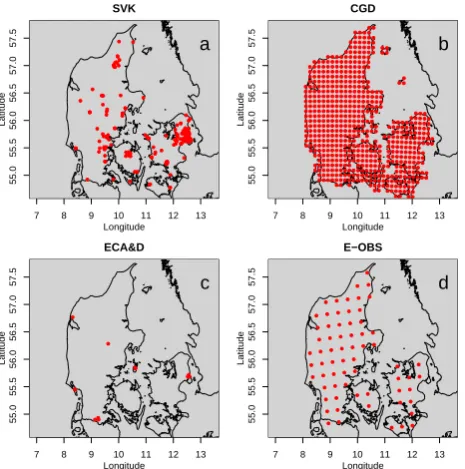
Four different observational data sets have been considered. These comprise two national data sets (SVK and Climate Grid Denmark (CGD)) and two freely available interna-tional data sets (European Climate Assessment and Dataset (ECA&D) and E-OBS). The SVK and ECA&D data are point measurements, while the CGD and E-OBS are gridded data sets. For this study all the data sets consist of daily pre-cipitation covering Denmark, and they are used as provided. Figure 1 shows the locations of the grid points and gauge lo-cations of the different data sets. This figure highlights the differences in the spatial distribution of the data available.
7 8 9 10 11 12 13
55.0
55.5
56.0
56.5
57.0
57.5
SVK
Longitude
Latitude
a
7 8 9 10 11 12 13
55.0
55.5
56.0
56.5
57.0
57.5
CGD
Longitude
Latitude
b
7 8 9 10 11 12 13
55.0
55.5
56.0
56.5
57.0
57.5
ECA&D
Longitude
Latitude
c
7 8 9 10 11 12 13
55.0
55.5
56.0
56.5
57.0
57.5
E−OBS
Longitude
Latitude
[image:4.595.52.285.63.298.2]d
Fig. 1. Location of grid points and gauges of the observational data
sets used. (a) Gauge locations of the Danish SVK gauge system, (b) grid locations of the regular 10 km grid in the Climate Grid Den-mark (CGD), (c) gauge locations included in the ECA&D and (d) grid locations of the 25 km rotated grid used by the E-OBS and the climate models.
1979 to 2012, and the spatial coverage is centred on the most urbanized areas of Denmark. Due to its purpose, the SVK data set is operated with a rather high threshold for dry weather, i.e. hours with less than approximately 0.2–0.4 mm of rain are considered dry (Jørgensen et al., 1998). For this study the daily precipitation values are calculated from the base data set. The SVK gauge locations are shown in Fig. 1a. CGD is a gridded precipitation product created by the Danish Meteorological Institute (DMI). It presents daily precipitation based on approximately 300 stations covering Denmark in an irregular but relatively homogeneous, dense network (Scharling, 1999). The station data has been interpo-lated in grids of 10×10 km using an inverse distance weight-ing method (Scharlweight-ing, 1999, 2012). The data set has only recently been released for research purposes, and the qual-ity of both the station data and the resulting gridded data has been extensively studied by DMI and found to be very good (Scharling, 2000; Scharling and Kern-Hansen, 2002). The data set is available for 1989 to 2010. The CGD grid locations are shown in Fig. 1b.
ECA&D is a large pan-European station data set that con-tains more than 2000 stations measuring daily precipitation (Klein Tank et al., 2002; Klok and Klein Tank, 2009). In Denmark, there are a total of 26 stations of which 17 are available for downloading from the project website (http: //www.ecad.eu). The period covered by the time series varies depending on the station. The stations available in Denmark
cover a period of more than 30 yr and all of them are cur-rently operational.
The ECA&D data is used as a basis to obtain the grid-ded data set E-OBS (Haylock et al., 2008). This data set was created as part of the ENSEMBLES project (van der Linden and Mitchell, 2009) and covers the time period 1951–2012. The means used to obtain the gridded data based on point measurements is a kriging method presented by Haylock et al. (2008). The E-OBS data set is available at a resolution of 0.22 and 0.44◦ (approximately 25 and 50 km, respectively) both in a regular latitude-longitude grid and a rotated pole grid. In this study we use version 5.0 of the rotated pole grid data set at a resolution of 0.22◦. At this resolution there are 66 land grids over Denmark. Both ECA&D and E-OBS have been widely used in climate change impact studies (Boberg et al., 2009, 2010; Christensen et al., 2010; Kjellström et al., 2010; Lenderink, 2010). E-OBS is regularly updated and the number of stations included is increasing. However, the number of stations in some regions is currently low com-pared to the number of grid points. The low density of sta-tions in some regions leads to an over-smoothing of precip-itation intensities, and especially of extreme events (Hofstra et al., 2009, 2010). The ECA&D gauge locations are shown in Fig. 1c and the E-OBS grid locations in Fig. 1d.
2.2 Climate model data
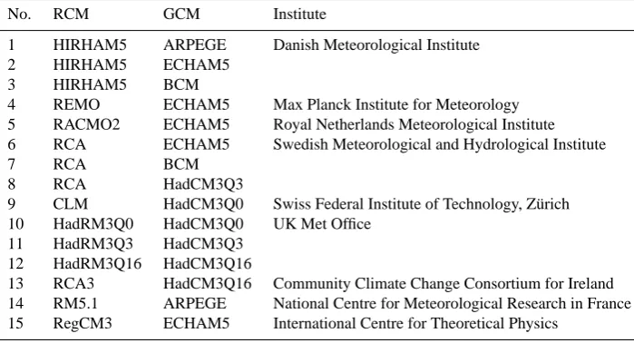
The four observational data sets are compared with a multi-model ensemble of RCMs from the European ENSEMBLES project. The project aimed at developing an ensemble predic-tion system to assess the uncertainty in climate projecpredic-tions from seasonal to decadal and longer timescales (van der Lin-den and Mitchell, 2009). A large data set of RCMs based on several GCMs was set up as part of the ENSEMBLES project. In this study we consider 15 RCMs driven by 6 dif-ferent GCMs. Table 1 shows the RCMs considered, where the number assigned to each of the RCMs will be used in the results sections.
Table 1. List of RCMs used in this study, driving GCMs and source of the RCMs.
No. RCM GCM Institute
1 HIRHAM5 ARPEGE Danish Meteorological Institute
2 HIRHAM5 ECHAM5
3 HIRHAM5 BCM
4 REMO ECHAM5 Max Planck Institute for Meteorology
5 RACMO2 ECHAM5 Royal Netherlands Meteorological Institute
6 RCA ECHAM5 Swedish Meteorological and Hydrological Institute
7 RCA BCM
8 RCA HadCM3Q3
9 CLM HadCM3Q0 Swiss Federal Institute of Technology, Zürich
10 HadRM3Q0 HadCM3Q0 UK Met Office
11 HadRM3Q3 HadCM3Q3
12 HadRM3Q16 HadCM3Q16
13 RCA3 HadCM3Q16 Community Climate Change Consortium for Ireland
14 RM5.1 ARPEGE National Centre for Meteorological Research in France
15 RegCM3 ECHAM5 International Centre for Theoretical Physics
3 Methodology
This study is divided into two main parts. The first part con-sists of an inter-comparison of indices from the different ob-servational data sets. The comparison is based on the abso-lute value of the indices and their spatial pattern. The second part compares the climate model performance estimated us-ing each of the different observational data sets. The climate model performance is assessed using two different metrics, which are applied to all the indices. This section describes the indices considered in the study and the metrics used to assess the climate model performance.
3.1 Indices
3.1.1 Point and grid point
A set of indices is used to compare the different observa-tional data sets and RCM outputs. The indices are chosen to represent information often evaluated in climate studies. They represent a range of temporal scales as well as mean and extreme precipitation properties. The indices evaluated are:
– The mean annual precipitation (Mean).
– The proportion of dry days (PDD).
– The simple daily intensity index (SDII) which is the
same as the mean precipitation amount per wet day.
– The 75th, 90th, 95th, 97.5th and 99th percentiles of the
wet days precipitation amount (Prec75p to Prec99p). Both the SDII and Prec90p are in the list of core indices de-fined by ETCCDI. Wet days are dede-fined as days with precip-itation higher or equal to 1 mm (Peterson, 2005; Seneviratne et al., 2012). These indices are estimated separately for each
of the stations in the observational point measurement data sets and for each grid point in the observational gridded data sets and the RCMs.
3.1.2 Spatial pattern
The set of indices defined above are also used to investigate the differences in the spatial pattern of the different data sets. Empirical semivariograms are used for this purpose. Empir-ical semivariograms use the value of the index at each point to estimate the semivariance, i.e. how the similarity between points changes with distance. This allows us to investigate the spatial pattern of each of the indices described above.
Semivariograms show the value of the semivariance de-pending on the distance (lag) between points. The semivari-ance,γ (d), is a measure of dissimilarity between two points separated in space by distanced. The semivariance increases with distance until it levels off. The distance at which the semivariogram levels off is known as the range. Two points are considered to be uncorrelated if they are at a distance equal to or higher than the range, also known as the decorre-lation length. The semivariance at a distanced is estimated by Wackernagel (2003) as:
2γ (d)=En[Z (x)−Z (x+d)]2o (1)
whereZ(x)is the value of the index at the pointx, andZ(x+
shown in Eq. (1). Empirical semivariograms are constructed for each of the observational data sets and for the RCMs.
Empirical semivariograms have been previously used in climate studies to rank RCMs according to their performance in reproducing spatial patterns (e.g. Fowler and Ekström, 2009). For this reason and due to their ability to represent the spatial pattern of a specific index, they have been selected in this study to assess the performance of the RCMs. Nonethe-less, a more concise summary of the similarity between spa-tial patterns can be graphically shown using Taylor diagrams (see Taylor (2001) for details). The Taylor diagrams show three metrics. They show the centred root mean square dif-ference (RMSD) and the spatial correlation between model data and observations. Additionally, they show the spatial standard deviation of the model data and observations. Taylor diagrams were specifically developed to summarize statisti-cal information of how well patterns match. Hence, Taylor diagrams have been used here to further compare the spatial pattern of the RCMs with the observational data sets.
3.2 Metric
In the second part of the analysis, the performance of the RCMs is assessed by comparing the indices estimated for the observational data sets to the indices estimated from the RCM outputs.
3.2.1 Point and grid point
The first metric used is based on the bias in reproducing the precipitation indices. The bias is calculated individually for each grid point in the RCMs for which observational data is available. It is estimated by subtraction of observations from the RCM output, i.e. a positive bias indicates that the RCM output yields higher indices than the observations. The abso-lute value of the median of the bias is then used to rank the RCMs, i.e. the climate model with the smallest median of the bias is ranked in first position.
3.2.2 Spatial pattern
The second metric used to assess the performance of the cli-mate models is based on the representation of the spatial pattern. The empirical semivariograms are used for this pur-pose. The performance of the RCMs is assessed using the root mean square error (RMSE). For each climate model, the error at a specific lag is calculated as the difference between the semivariance estimated from the climate model and the observations. The RMSE for the modelmis then calculated as
RMSEm=
r
1
N
XN
i=1 γ
m
i −γ
Obs
i
2
, (2)
whereγiObsandγimare the semivariance for the observations and climate modelmat lagi, respectively.N is the number
of bins in the semivariogram. The model with the smallest RMSE is ranked in first position. It must be highlighted that the comparison of the climate models is carried out using the empirical semivariance. We do not attempt to parameterise the semivariogram, as often done in interpolation methods. This would include additional uncertainties arising from both the model selection and the parameter estimation.
In addition to using the spatial pattern for assessing the performance of the RCMs, it is also used to assess the sim-ilarities of the RCMs in the ensemble. This is of relevance when using the ensemble of RCMs to quantify the uncer-tainty in climate change projections. Most unceruncer-tainty quan-tification techniques assume that the models are independent. However, this assumption may not be valid as some models may share part of code, parameterizations and/or are driven by the same GCMs. The validity of this assumption is ad-dressed in detail by Tebaldi and Knutti (2007), Knutti et al. (2010), and Pennell and Reichler (2011). In a recent study by Sunyer et al. (2013) the interdependency of the ENSEM-BLES RCMs over Denmark is investigated using E-OBS as the observational data set. The impact of the observational data set chosen is investigated in this study.
The methodology followed here is the same as in Sunyer et al. (2013). The first step is the estimation of the metric to investigate the interdependency of RCMs. The metric used is a measure of the model error. It is estimated by removing the ensemble average error from the individual model error. The ensemble average error represents the common biases. It is calculated separately for each grid point as the average of the model error of all the RCMs. For each index, the metric is estimated separately for all the grid points for each RCM in the ensemble.
The similarity of the RCMs can then be assessed using a hierarchical cluster analysis (Wilks, 2006). This analysis groups the RCMs into clusters depending on their similar-ity. The similarity of the RCMs is expressed by means of the correlation matrix, R, the elements of which are the correla-tions between the metric estimated for all the RCMs. Den-drograms are used to illustrate the results of the hierarchical cluster analysis. The dendrograms show the dissimilarity of the RCMs, estimated as the Pearson’s distance, i.e. 1−R.
4 Results and discussions
4.1 Comparison of observational data sets
4.1.1 Point and grid point
Fig. 2. The mean precipitation (Mean) of Denmark for CGD (left)
and E-OBS (right).
drier than CGD in the eastern part and for most of the western part, except for the most southern grid points. E-OBS is also drier than CGD in the middle-eastern grid points of Jutland and the most northern grid points.
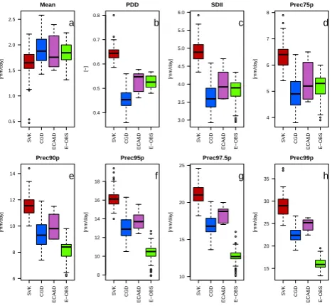
The box plots in Fig. 3 summarize the indices estimated for each point for all the data sets. The boxes represent the 25th, 50th and 75th percentiles, the whiskers represent the 5th and 95th percentile, and the circles show the outliers. The box plot for the mean, Fig. 3a, shows a good agree-ment among the data sets. The median ranges between 600 and 700 mm yr−1(approximately 1.6 and 2 mm day−1as pre-sented by the mean), the total span is of a few hundred mm yr−1(approximately 1 to 1.2 mm day−1). This is the ex-pected range of mean precipitation for Denmark as deter-mined by historical investigations (Frich et al., 1997; Madsen et al., 2009). The SVK data set has the lowest median of all the data sets. This is expected to be an artefact mainly caused by the relatively high threshold used in the processing (Jør-gensen et al., 1998). The box plot of the other long temporal scale index, PDD, shows larger differences between the data sets (see Fig. 3b). In this case the SVK data set also stands out with a considerably larger PDD than the other data sets. The differences are likely to be due to the same phenomena as in the mean. The high threshold for the SVK data should result in absolutely no drizzling and an increased PDD.
As in the case of the mean and PDD, for the SDII and Prec75p only the SVK data set stands notably out. It has a considerably higher median value but comparable variation. Again, this is most likely linked to the high threshold that leads to fewer wet days. In the case of the higher percentiles, there is a tendency to larger differences between the data sets. Point measurement data sets show higher values than the gridded data sets. Additionally, the gridded data set with a higher spatial resolution (CGD) shows higher values than the gridded data set with a lower spatial resolution (E-OBS). This is in agreement with the general understanding that the gridding of point measurements tends to smooth out extreme precipitation (Chen and Knutson, 2008; Hofstra et al., 2010). The difference between the ECA&D data set and the CGD data set seems to be in the expected range of a 15–20 % re-duction in intensity from point scale to a 100 km2grid that could be explained by the simple ARF (Wilson, 1990). The
SVK CGD ECA&D E−OBS
0.5 1.0 1.5 2.0 2.5
Mean
[mm/da
y]
a
SVK CGD ECA&D E−OBS
0.4 0.5 0.6 0.7 0.8
PDD
[−]
b
SVK CGD ECA&D E−OBS
3.0 3.5 4.0 4.5 5.0 5.5 6.0
SDII
[mm/da
y]
c
SVK CGD ECA&D E−OBS
4 5 6 7 8
Prec75p
[mm/da
y]
d
SVK CGD ECA&D E−OBS
6 8 10 12 14
Prec90p
[mm/da
y]
e
SVK CGD ECA&D E−OBS
8 10 12 14 16 18
Prec95p
[mm/da
y]
f
SVK CGD ECA&D E−OBS
10 15 20 25
Prec97.5p
[mm/da
y]
g
SVK CGD ECA&D E−OBS
15 20 25 30 35
Prec99p
[mm/da
y]
[image:7.595.50.283.63.159.2]h
Fig. 3. Box plots summarising the mean precipitation (Mean) (a),
the proportion of dry days (PDD) (b), the mean precipitation amount per wet day (SDII) (c), and different percentiles of extreme precipitation (Prec75p to Prec99p) (d–h) for the four observational data sets.
E-OBS data set on the other hand is lower than expected by the ARF method (approximately 33 % reduction in intensity from point scale to 625 km2grid size) and the difference in-creases for higher percentiles.
The difference between CGD and E-OBS increases as a function of the percentile. This difference is believed to be partly due to the different spatial resolution and partly due to the amount of stations used in the gridding. CGD is cre-ated from roughly one observational station per grid cell, whereas E-OBS only has approximately one station available per three grid cells. The same difference is observed between the two point measurement observational data sets (SVK and ECA&D). Again it is believed to be a product of the dif-ference in the number and location of stations in the differ-ent data sets. The differences can hence be explained mainly by the quality of the underlying observational data, implying that having more gauges increase the chance of monitoring extremes.
4.1.2 Spatial pattern
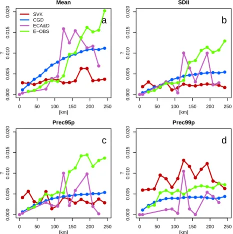
The spatial pattern of precipitation, which is of high impor-tance in hydrological applications, is assessed by calculat-ing empirical semivariograms for all the data sets. Figure 4 shows the semivariograms for the mean, SDII and the 95th and 99th percentiles. The maximum distance considered in the semivariograms is 250 km. This is due to the fact that the number of grid points available for higher distances are too few to obtain a reliable estimate of the semivariance. The semivariograms show that for the SVK data there is basically no spatial structure for all considered indices. Further, Fig. 4 shows that E-OBS has a marked increase in the semivari-ance with distsemivari-ance and no apparent range when compared with CGD. The difference in the spatial pattern of E-OBS and CGD could be explained by the difference in the number of stations used in these data sets. In E-OBS, precipitation measured at stations in the neighbouring countries is proba-bly assimilated into the grids for Denmark. Consequently, a higher semivariance would be obtained for E-OBS at large distances. The semivariograms of E-OBS and CGD do not level off at the same distance. This phenomenon is not ex-plicitly investigated further in the present study. It must also be noted that the two gridded data sets use different inter-polation methods; if the data basis is sufficient, this should only have minor influence on the result. Furthermore, due to Denmark’s flat topography daily precipitation values are ex-pected to vary slowly in space, and the effect of the interpola-tion method is expected to be small compared with the effect of the number of stations. The large number of stations can also explain the smoother semivariogram obtained for CGD. The high variation in ECA&D is probably due to the limited number of stations in this data set and along with the other point data set, SVK, a nugget effect due to the pooling of data is probably also influencing the semivariograms.
4.2 Climate model performance and ranking
The previous section has focused on comparing the absolute value and the spatial pattern of the indices of different ob-servational data sets. These data sets could all potentially be used for defining the baseline climate in climate change impact studies in Denmark, and in fact SVK, ECA&D and E-OBS have been used for this purpose (e.g. Boberg et al., 2009, 2010; Lenderink, 2010; Sunyer et al., 2012; Gregersen et al., 2013). This section assesses the performance of the cli-mate models using the four different observational data sets analysed in the previous section. The bias in the point indices and the RMSE in the empirical semivariograms are the met-rics used to rank the climate models. The indices estimated using CGD have been re-interpolated into the same grid sys-tem as E-OBS and the RCMs. This is done to be able to compare the results obtained using CGD and E-OBS with-out the effect of the spatial resolution. The re-interpolation method used is the same as the one used for the RM5.1 and
0 50 100 150 200 250
0.000
0.005
0.010
0.015
0.020
Mean
[km]
γ
SVK CGD ECA&D E−OBS
a
0 50 100 150 200 250
0.000
0.005
0.010
0.015
0.020
SDII
[km]
γ
b
0 50 100 150 200 250
0.000
0.005
0.010
0.015
0.020
Prec95p
[km]
γ
c
0 50 100 150 200 250
0.000
0.005
0.010
0.015
0.020
Prec99p
[km]
γ
[image:8.595.311.545.65.300.2]d
Fig. 4. Semivariograms of the mean precipitation (mean) (a), the
mean precipitation amount per wet day (SDII) (b), and the differ-ent percdiffer-entiles of extreme precipitation (Prec95p and Prec99p) (c,
d) for all observational data sets showing the difference in spatial
patterns.
RegCM3 models. The re-interpolated CGD data is referred to as CGD-25.
4.2.1 Point and grid point
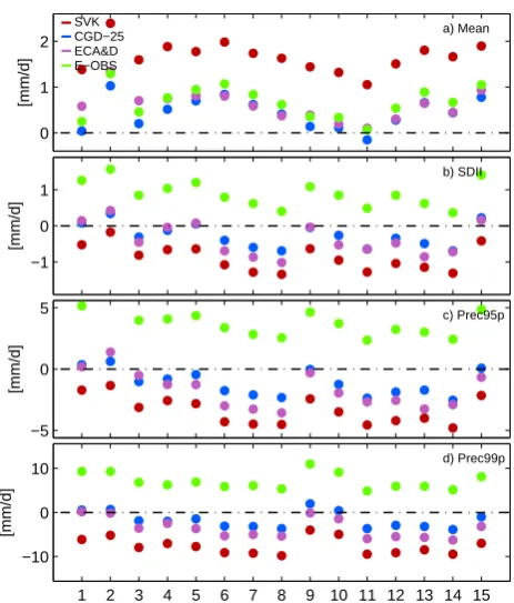
Figure 5 shows the value of the median of the bias of each of the 15 RCMs in the ensemble calculated using each of the ob-servational data sets. For all the indices the bias estimated is highly dependent on the observational data used. In the case of the mean precipitation, the bias estimated using CGD-25 is lower than the bias estimated using the other observational data sets. On the other hand, the highest biases are obtained when using the SVK data as the observational data set. This is in agreement with the lower values of the mean precipita-tion found for this observaprecipita-tional data set in Fig. 3. The biases estimated using ECA&D and E-OBS are rather similar to the bias estimated using CGD-25, the difference is smaller than 0.5 mm day−1. However, E-OBS leads to slightly higher bias
for most RCMs. Nonetheless, for most of the climate models the observational data sets agree on the positive sign of the bias, i.e. the RCMs overestimate the mean precipitation.
In general, the SVK, CGD-25, and ECA&D point to an un-derestimation of SDII, Prec95p, and Prec99p by the RCMs, while E-OBS points to an overestimation. For these three in-dices, the bias estimated using the gridded observational data sets is, in most cases, higher than the bias estimate using the point observational data sets. This is due to the lower value of these indices found for the gridded observational data sets (see Fig. 3). As expected, and in agreement with the results from the previous section, the difference between the biases is higher for higher percentiles.
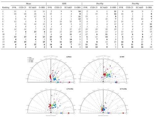
Table 2 shows the ranking of the 15 RCMs according to the metric based on the bias and for four of the indices (mean, SDII, Prec95p and Prec99p). In this table the num-ber assigned to each RCM corresponds to the enumeration used in Table 1. The differences observed in Fig. 5 stand out in the ranking of the models. In the case of the mean, the same models are ranked in the highest positions for all the observational data sets. The five models with the high-est ranking for the SVK data set (models highlighted in ro-man in Table 2) are among the seven best models for CGD-25, ECA&D and E-OBS. A similar pattern is observed for the models with the lowest ranking (models highlighted in bold). However, for the other three indices (SDII, Prec95p and Prec99p) the rankings are more dissimilar. For example, for Prec95p, model 2 has rank 1 in the SVK data but rank 5, 7 and 15 for the CGD-25, ECA&D and E-OBS, respectively. In general, the SVK, CGD-25 and ECA&D data sets lead to more similar model rankings, whereas E-OBS tends to have a reverse ranking. This can be explained by the difference in the sign of the bias when using E-OBS and when using SVK, ECA&D, and CGD-25. In general, the values of SDII, Prec95p and Prec99p of the RCMs lay between the values estimated using E-OBS and SVK, ECA&D, and CGD. This implies that when the absolute value of the bias of an RCM is small according to E-OBS it is found large according to SVK, ECA&D, and CGD.
4.2.2 Spatial pattern
The previous results compare the RCMs with the observa-tional data sets based on the value of the indices at point measurements and grid points. This section focuses on the ability of the RCMs to reproduce the spatial pattern in the observational data sets.
Figure 6 shows the Taylor diagrams for the mean, SDII, Prec95p and Prec99p indices. For all the indices and in most cases, the standard deviation of the RCMs is lower than the standard deviation of the observational data sets. The larger differences between the spatial variability of the RCMs in the ensemble are found when using ECA-D as the observational data set. Similarly, the larger difference between RCMs and the observational data set are found for the SVK data. This observational data set leads to higher spatial standard devi-ation than the other observdevi-ational data sets. As previously
0 1 2
[mm/d]
−1 0 1
[mm/d]
−5 0 5
[mm/d]
1 2 3 4 5 6 7 8 9 10 11 12 13 14 15 −10
0 10
[mm/d]
a) Mean
b) SDII
c) Prec95p
d) Prec99p SVK
[image:9.595.313.545.59.331.2]CGD−25 ECA&D E−OBS
Fig. 5. Bias of each of the RCMs in the ensemble estimated using
the four observational data sets. Model numbers are shown in Ta-ble 1.
mentioned, this is probably due to the heterogeneity of this data set.
The correlation of the RCMs with the different obser-vational data sets is slightly higher when comparing the RCMs with CGD-25. The RMSD estimated using CGD-25 is also slightly lower than the RMSD estimated using the other observational data sets. Nonetheless, both the correla-tion and RMSD of the RCMs are similar when using E-OBS and CGD-25. The RCMs show the smallest correlation and largest RMSD when compared with the SVK data set.
The Taylor diagrams show that performance of a specific model depends on the observational data set used. For exam-ple, the model represented with the filled square symbol has one of the highest correlations and lowest RMSD for all the indices for CGD-25 but not for the other observational data sets.
Table 2. Ranking of the RCMs depending on their bias for the observational data sets. Model numbers are shown in Table 1. The models
highlighted in roman, italic and bold refer to the models with rank 1 to 5, 6 to 10 and 11 to 15 for SVK, respectively.
Mean SDII Prec95p Prec99p
Ranking SVK CGD-25 ECA&D E-OBS SVK CGD-25 ECA&D E-OBS SVK CGD-25 ECA&D E-OBS SVK CGD-25 ECA&D E-OBS
1 11 1 11 11 2 9 9 14 2 9 1 11 9 10 9 5
2 10 10 10 1 15 5 4 8 1 15 9 14 10 1 1 8
3 1 9 12 10 1 1 5 11 15 1 3 8 2 2 2 6
4 9 11 8 9 9 4 1 13 9 5 15 7 1 15 10 7
5 12 3 9 3 5 15 15 7 4 2 5 13 15 5 4 4
6 3 12 14 12 4 10 2 6 5 4 4 12 4 3 15 11
7 8 8 1 8 3 3 3 3 3 3 2 6 5 9 3 14
8 14 14 7 14 10 2 12 12 10 10 10 10 3 4 5 12
9 7 4 13 4 12 12 10 10 13 13 12 3 13 12 7 15
10 5 7 3 7 6 6 11 4 12 6 11 4 12 6 6 3
11 13 13 4 13 13 13 6 9 6 12 14 5 6 13 8 13
12 4 5 6 5 11 7 14 5 7 7 6 9 7 7 12 2
13 15 15 5 15 7 11 13 1 8 8 13 15 14 8 13 1
14 6 6 15 6 14 8 7 15 11 11 7 1 11 11 11 9
15 2 2 2 2 8 14 8 2 14 14 8 2 8 14 14 10
0.2 0.4 0.6 0.8
0 0.2 0.4 0.6 0.8 −1
−0.8 −0.6
−0.4
−0.2 0 0.2 0.4
0.6
0.8
1 0.95
0.99 −0.95
−0.99
Cor re l at i on Coef f i c i ent
0.2 0.4 0.6
0 0.2 0.4 0.6 −1
−0.8 −0.6
−0.4
−0.2 0 0.2 0.4
0.6
0.8
1 0.95
0.99 −0.95
−0.99
Cor re l at i on Coef f i c i ent
0.5 1 1.5 2
0 0.5 1 1.5 2 −1
−0.8 −0.6
−0.4
−0.2 0 0.2 0.4
0.6
0.8
1 0.95
0.99 −0.95
−0.99
Standard deviation
2 4 6
0 2 4 6
−1 −0.8
−0.6 −0.4
−0.2 0 0.2 0.4
0.6
0.8
1 0.95
0.99 −0.95
−0.99
Standard deviation
a) Mean b) SDII
c) Prec95p d) Prec99p
SVK CGD−25 ECA&D E−OBS
Fig. 6. Taylor diagrams showing the spatial correlation, centred RMSD, and the standard deviation for each of the RCMs when compared
with each of the observational data sets (represented with stars in the line of correlation equal to 1). The different colours represent the observational data set used as a reference and the different markers show each of the RCMs in the ensemble. The values of the RMSD are shown using the SVK data set as a reference. For simplicity, the values of the RMSD for the other observational data sets are not shown.
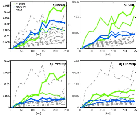
In the case of the mean, the model with the smallest RMSE is the same for the two observational data sets (model RACMO2 driven by ECHAM5, model 5 in Table 1). How-ever, for SDII, Prec95p and Prec99p the model with the smallest RMSE depends on the observational data set used. In agreement with spatial standard deviation shown in the Taylor diagrams, in general, the RCMs show a smaller semi-variance than the observational data sets for all the indices.
The difference in the spatial pattern of the gridded obser-vational data sets also has an effect on the interpretation of the information available in the ensemble of RCMs. Figure 8 shows the ensemble average error and the dendrograms for Prec95p estimated using E-OBS and CGD-25. They axis in the dendrograms is the Pearson’s distance, which is a
mea-sure of dissimilarity of the RCMs. All the RCMs included in the ensemble are shown in thexaxis. The ensemble average error represents the common biases in the ensemble, while the dendrograms show the clustering of the RCMs.
0 50 100 150 200 250 0
0.005 0.01 0.015 0.02 0.025 0.03
0.035 a) Mean
[km]
γ
0 50 100 150 200 250 0
0.005 0.01 0.015
b) SDII
[km]
γ
0 50 100 150 200 250 0
0.005 0.01 0.015 0.02
c) Prec95p
[km]
γ
0 50 100 150 200 250 0
0.005 0.01 0.015 0.02
d) Prec99p
[km]
γ
[image:11.595.310.542.63.218.2]E−OBS CGD−25 RCM
Fig. 7. Semivariograms for E-OBS, CGD-25 and all the RCMs. The
RCMs with the minimum RMSE estimated using E-OBS and CGD-25 are highlighted in green and in blue, respectively.
which in turn lead to differences in the correlation matrix, R. This is reflected in the dendrograms. For example, in the den-drogram using E-OBS, the RACMO2 model (model 5) forms a cluster with the three HIRHAM models (models 1, 2, and 3), while in the dendrogram using CGD-25 this model forms a cluster with the models from the Hadley Centre (models 10, 11, and 12). Nonetheless, there are also some common re-sults in the dendrograms. The most relevant one being that the same RCM driven by different GCMs (i.e. HIRHAM, RCA and HadRM models) are more similar than different RCMs driven by the same GCM.
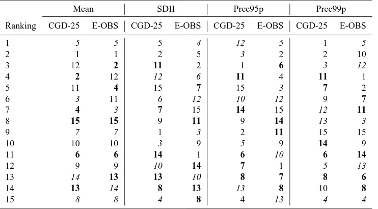
Table 3 shows the ranking of the climate models accord-ing to the RMSE of the semivariograms. As seen in Table 3, the model with the highest ranking in mean precipitation is the same for both observational data sets (model 5). For this index the RCMs have virtually similar ranking for the two observational data sets. The difference between the rankings increases from SDII to Prec99p. It must be noted that the ranking of the RCMs based on the semivariograms obtained for CGD-25 and E-OBS is more similar than the ranking ob-tained using the bias at the grid points for these two observa-tional data sets.
[image:11.595.51.284.64.257.2]It must also be noted that the ranking of the models us-ing the same observational data set varies dependus-ing on the index. This is observed both in Table 2 and Table 3. Simi-larly, for the same observational data set the ranking of the model also varies depending on the metric used. For exam-ple in the case of E-OBS, the best model at representing the spatial pattern (model 5) for Prec95p is ranked in eleventh position regarding the bias. These results show that the per-formance of the models depends on the index and metric of interest. Therefore, it is not possible to generally classify the models as good or bad models. This is in agreement with the
Fig. 8. Ensemble average error (a, b) and dendrograms (c, d) for
Prec95p estimated using CGD-25 (a, c) and E-OBS (b, d). They
axis in the dendrograms shows the dissimilarity of the climate mod-els. Model numbers are shown in Table 1.
results from previous studies, e.g. Lenderink (2010), Kjelll-ström et al. (2010). The dependency of the ranking on the index and the metric highlights the importance of using an ensemble of RCMs to obtain robust climate projections for future climate conditions.
5 Conclusions
This study investigates the influence of the choice of obser-vational data set in the assessment of climate model per-formance. Four different observational data sets have been analysed. These represent the common type of observations used in climate change impact studies (point measurement and gridded data). A set of indices (ranging from the mean to high percentiles) and two different metrics (based on bias and root mean square error of spatial patterns) are used to analyse and compare daily precipitation data from observational data sets and from an ensemble of RCMs.
Table 3. Ranking of the RCMs depending on the RMSE of the semivariograms for the observational data sets. Model numbers are shown in
Table 1. The models highlighted in roman, italic and bold correspond to the models with rank 1 to 5, 6 to 10 and 11 to 15 for SVK in Table 2, respectively.
Mean SDII Prec95p Prec99p
Ranking CGD-25 E-OBS CGD-25 E-OBS CGD-25 E-OBS CGD-25 E-OBS
1 5 5 5 4 12 5 1 5
2 1 1 2 5 3 2 2 10
3 12 2 11 2 1 6 3 12
4 2 12 12 6 11 4 11 1
5 11 4 15 7 15 3 7 2
6 3 11 6 12 10 12 9 7
7 4 3 7 15 14 15 12 11
8 15 15 9 11 9 14 13 3
9 7 7 1 3 2 11 15 15
10 10 10 3 9 5 9 14 9
11 6 6 14 1 6 10 6 14
12 9 9 10 14 7 1 5 13
13 14 13 13 10 8 7 8 6
14 13 14 8 13 13 8 10 8
15 8 8 4 8 4 13 4 4
especially extreme precipitation, resulting in less intense ex-tremes in comparison to the other observational data sets. The different data sets also show different spatial patterns. Even though it over-smoothes the precipitation intensities, E-OBS shows a lower correlation of the grid points at large distances than the CGD data.
The differences identified between the observational data sets are important when assessing climate model perfor-mance. This is clearly shown in the analysis of the bias, where the sign of the bias for high percentiles is different when comparing the RCMs to E-OBS or to SVK, CGD-25 and ECA-D. Furthermore, the ranking of the climate models is almost opposite when considering E-OBS vs. SVK, CGD-25 and ECA-D data sets. In the case of the mean precipita-tion, the ranking is less dependent on the observational data set considered, probably because it is an index that is robust to spatial and temporal averaging.
Similar conclusions can be drawn from the analysis of the spatial pattern. The ranking of the climate models depends both on the observational data set used and on the index. Higher differences between the rankings are observed for ex-treme precipitation. The differences in the spatial pattern of the gridded observational data sets also affect the conclusions regarding the similarity of the RCM biases. Additionally, as other studies have also stressed, when considering only one of the observational data sets, the ranking of the climate mod-els depends on the index and metric used to rank the modmod-els. The results of this study illustrate and highlight the need to be aware of the different characteristics of observational data sets, as this has a high influence on the performance es-timated for each of the RCMs. RCMs should be compared to quality-checked observational data that represents the same
precipitation characteristics. In this study the data set that better fits these requirements is the CGD data re-interpolated to the same grid resolution as the RCMs, i.e. CGD-25. Fur-ther work should focus on addressing the possible errors and uncertainty (e.g. measurement and interpolation uncertainty) in the observations, especially if the interest of the study is mainly in extreme precipitation.
Acknowledgements. This work was carried out with the support of the Danish Council for Strategic Research as part of the project RiskChange, contract no. 10-093894 (http://riskchange.dhigroup. com), and with the support of the Danish Council for Independent Research as part of the project “Reducing Uncertainty of Future Ex-treme Precipitation”, contract no. 09-067455.
The Climate Grid Denmark data set is a product of the Danish Meteorological Institute and the SVK data set a product of The Water Pollution Committee of The Society of Danish Engineers. The data from the RCMs and E-OBS used in this work was funded by the EU FP6 Integrated Project ENSEMBLES contract number 05539 (http://ensembles-eu.metoffice.com) and the data providers in the ECA&D project (http://eca.knmi.nl), whose support is gratefully acknowledged.
Edited by: A. Langousis
References
Bárdossy, A. and Pegram, G.: Downscaling precipitation using re-gional climate models and circulation patterns toward hydrology, Water Resour. Res., 47, W04505, doi:10.1029/2010WR009689, 2011.
based on two methods for transferring regional climate model results to meteorological station sites, Tellus A, 60, 439–450, doi:10.1111/j.1600-0870.2008.00306.x, 2008.
Benestad, R. E.: Downscaling precipitation extremes, Theor. Appl. Climatol., 100, 1–21, doi:10.1007/s00704-009-0158-1, 2010. Beniston, M., Stephenson, D., Christensen, O., Ferro, C., Frei, C.,
Goyette, S., Halsnaes, K., Holt, T., Jylhä, K., Koffi, B., Palutikof, J., Schöll, R., Semmler, T., and Woth, K.: Future extreme events in European climate: an exploration of regional climate model projections, Climatic Change, 81, 71–95, doi:10.1007/s10584-006-9226-z, 2007.
Boberg, F. and Christensen, J. H.: Overestimation of
Mediterranean summer temperature projections due to
model deficiencies, Nature Climate Change, 2, 433–436, doi:10.1038/NCLIMATE1454, 2012.
Boberg, F., Berg, P., Thejll, P., Gutowski, W., and Christensen, J. H.: Improved confidence in climate change projections of pre-cipitation evaluated using daily statistics from the PRUDENCE ensemble, Clim. Dynam., 32, 1097–1106, doi:10.1007/s00382-008-0446-y, 2009.
Boberg, F., Berg, P., Thejll, P., Gutowski, W., and Christensen, J. H.: Improved confidence in climate change projections of precipita-tion further evaluated using daily statistics from ensembles mod-els, Clim. Dynam., 35, 1509–1520, doi:10.1007/s00382-009-0683-8, 2010.
Burton, A., Fowler, H. J., Blenkinsop, S., and Kilsby, C. G.: Down-scaling transient climate change using a Neyman–Scott Rectan-gular Pulses stochastic rainfall model, J. Hydrol., 381, 18–32, doi:10.1016/j.jhydrol.2009.10.031, 2010.
Chen, C.-T. and Knutson, T.: On the Verification and Comparison of Extreme Rainfall Indices from Climate Models, J. Climate, 21, 1605–1621, doi:10.1175/2007JCLI1494.1, 2008.
Christensen, N. S. and Lettenmaier, D. P.: A multimodel ensem-ble approach to assessment of climate change impacts on the hydrology and water resources of the Colorado River Basin, Hy-drol. Earth Syst. Sci., 11, 1417–1434, doi:10.5194/hess-11-1417-2007, 2007.
Christensen, J. H., Kjellström, E., Giorgi, F., Lenderink, G., and Rummukainen, M.: Weight assignment in regional climate mod-els, Clim. Res., 44, 179–194, doi:10.3354/cr00916, 2010. Cooley, D. and Sain, S. R.: Spatial Hierarchical Modeling of
Precip-itation Extremes From a Regional Climate Model, J. Agric. Biol. Envir. S., 15, 381–402, doi:10.1007/s13253-010-0023-9, 2010. Dai, A., Meehl, G. A., Washington, W. M., Wigley, T. M., and
Ar-blaster, J. M.: Ensemble simulation of twenty-first century
cli-mate changes: Bussiness-as-usual versu CO2 Stabilization, B.
Am. Meteorol. Soc., 82, 2377–2388, 2001.
De Michele, C., Kottegoda, N. T., and Rosso, R.: The derivation of areal reduction factor of storm rainfall from its scaling properties, Water Resour. Res., 37, 3247–3252, doi:10.1029/2001WR000346, 2001.
De Michele, C., Kottegoda, N. T., and Rosso, R.: IDAF (intensity-duration-area frequency) curves of extreme storm rainfall: a scal-ing approach, Water Sci. Technol., 45, 83–90, 2002.
De Michele, C., Zenoni, E., Pecora, S., and Rosso, R.: Ana-lytical derivation of rain intensity-duration-area-frequency re-lationships from event maxima, J. Hydrol, 399, 385–393, doi:10.1016/j.jhydrol.2011.01.018, 2011.
Déqué, M., Rowell, D., Lüthi, D., Giorgi, F., Christensen, J., Rockel, B., Jacob, D., Kjellström, E., de Castro, M., and van den Hurk, B.: An intercomparison of regional climate simulations for europe: assessing uncertainties in model projections, Climatic Change, 81, 53–70, doi:10.1007/s10584-006-9228-x, 2007. Dessai, S. and Hulme, M.: Assessing the robustness of adaptation
decisions to climate change uncertainties: A case study on water resources management in the east of England, Global Environ. Chang., 17, 59–72, doi:10.1016/j.gloenvcha.2006.11.005, 2007. Fankhauser, R.: Influence of systematic errors from tipping bucket rain gauges on recorded rainfall data, Water Sci. Technol., 37, 121–129, doi:10.1016/S0273-1223(98)00324-2, 1998.
Fatichi, S., Ivanov, V. Y., and Caporali, E.: Simulation of future cli-mate scenarios with a weather generator, Adv. Water Resour., 34, 448–467, 2011.
Fowler, H. J. and Ekström, M.: Multi-model ensemble estimates of climate change impacts on UK seasonal precipitation extremes, Int. J. Climatol., 29, 385–416, doi:10.1002/joc.1827, 2009. Frei, C., Christensen, J. H., Déqué, M., Jacob, D., Jones, R. G.,
and Vidale, P. L.: Daily precipitation statistics in regional climate models: Evaluation and intercomparison for the European Alps, J. Geophys. Res., 108, 4124, doi:10.1029/2002JD002287, 2003. Frei, C., Schöll, R., Fukutome, S., Schmidli, J., and Vidale, P. L.: Future change of precipitation extremes in europe: Intercompari-son of scenarios from regional climate models, J. Geophys. Res., 111, D06105, doi:10.1029/2005JD005965, 2006.
Frich, P., Rosenørn, S., Madsen, H., and Jensen, J. J.: Observed Pre-cipitation in Denmark 1961–90, Technical Report number 97-8 available at www.dmi.dk, Danish Meteorological Institute, Den-mark, 1997.
Giorgi, F. and Mearns, L. O.: Calculation of average, uncer-tainty range, and reliability of regional climate changes from AOGCM simulations via the “reliability ensemble averaging” (rea) method, J. Climate, 15, 1141–1158, doi:10.1175/1520-0442(2002)015<1141:COAURA>2.0.CO;2, 2002.
Gómez-Navarro, J. J., Montávez, J. P., Jerez, S., Jiménes-Guerrero, P., and Zorita, E.: What is the role of the observational dataset in the evaluation and scoring of climate models?, Geophys. Res. Lett., 39, L24701, doi:10.1029/2012GL054206, 2012.
Goodess, C., Hall, J., Best, M., Betts, R., Cabantous, L., Jones, P., Kilsby, C., Pearman, A., and Wallace, C.: Climate scenarios and decision making under uncertainty, Built Environment, 33, 10– 30, 2007.
Gregersen, I. B., Sørup, H. J. D., Madsen, H., Rosbjerg, D., Mikkelsen, P. S., and Arnbjerg-Nielsen, K.: Assessing future climatic changes of rainfall extremes at small spatio-temporal scales, Climatic Change, 118, 783–797, doi:10.1007/s10584-012-0669-0, 2013.
Hanel, M. and Buishand, T. A.: On the value of hourly precipitation extremes in regional climate model simulations, J. Hydrol., 393, 265–273, doi:10.1016/j.jhydrol.2010.08.024, 2010.
Hawkins, E. and Sutton, R.: The potential to narrow uncertainty in projections of regional precipitation change, Clim. Dynam., 37, 407–418, doi:10.1007/s00382-010-0810-6, 2011.
Haylock, M. R., Hofstra, N., Klein Tank, A. M. G., Klok, E. J., Jones, P. D., and New, M.: A European daily high-resolution gridded dataset of surface temperature and precipitation, J. Geo-phys. Res., 113, D20119, doi:10.1029/2008JD010201, 2008. Hewitson, B. C. and Crane, R. G.: Gridded Area-Averaged Daily
Precipitation via Conditional Interpolation, J. Climate, 18, 41– 57, doi:10.1175/JCLI3246.1, 2005.
Hofstra, N., Haylock, M., New, M., and Jones, P. D.: Testing E-OBS European high-resolution gridded data set of daily precip-itation and surface temperature, J. Geophys. Res., 144, D21101, doi:10.1029/2009JD011799, 2009.
Hofstra, N., New, M., and McSweeney, C.: The influence of interpo-lation and station network density on the distributions and trends of climate variables in gridded daily data, Clim. Dynam, 35, 841– 858, doi:10.1007/s00382-009-0698-1, 2010.
Hundecha, Y. and Bárdossy, A.: Statistical downscaling of ex-tremes of daily precipitation and temperature and construc-tion of their future scenarios, Int. J. Climatol., 28, 589–610, doi:10.1002/joc.1563, 2008.
Iizumi, T., Nishimori, M., Dairaku, K., Adachi, S. A., and Yokozawa, M.: Evaluation and intercomparison of downscaled daily precipitation indices over Japan in present-day climate: Strengths and weaknesses of dynamical and bias correction-type statistical downscaling methods, J. Geophys. Res., 116, D01111, doi:10.1029/2010JD014513, 2011.
Jørgensen, H. K., Rosenørn, S., Madsen, H., and Mikkelsen, P. S.: Quality control of rain data used for urban runoff systems, Water Sci. Technol., 37, 113–120, doi:10.1016/S0273-1223(98)00323-0, 1998.
Kang, B. and Ramirez, J. A.: A coupled stochastic space-time inter-mittent random cascade model for rainfall downscaling, Water Resour. Res., 46, W10534, doi:10.1029/2008WR007692, 2010. Kjellström, E., Boberg, F., Castro, M., Christensen, J. H., Nikulin,
G., and Sánchez, E.: Daily and monthly temperature and precip-itation statistics as performance indicators for regional climate models, Clim. Res., 44, 135–150, doi:10.3354/cr00932, 2010. Klein Tank, A. M. G., Wijngaard, J. B., Können, G. P., Böhm, R.,
Demarée, G., Gocheva, A., Mileta, M., Pashiardis, S., Hejkr-lik, L., Kern-Hansen, C., Heino, R., Bessemoulin, P., Müller-Westermeier, G., Tzanakou, M., Szalai, S., Pálsdóttir, T., Fitzger-ald, D., Rubin, S., Capaldo, M., Maugeri, M., Leitass, A., Bukan-tis, A., Aberfeld, R., van Engelen, A. F. V., Forland, E., Mietus, M., Coelho, F., Mares, C., Razuvaev, V., Nieplova, E., Cegnar, T., Antonio López J., Dahlström, B., Moberg, A., Kirchhofer, W., Ceylan, A., Pachaliuk, O., Alexander, L. V., and Petrovic, P.: Daily dataset of 20th-century surface air temperature and pre-cipitation series for the European Climate Assessment, Int. J. Cli-matol., 22, 1441–1453, doi:10.1002/joc.773, 2002.
Klok, E. J. and Klein Tank, A. M. G.: Updated and extended Euro-pean dataset of daily climate observations, Int. J. Climatol., 29, 1182–1191, doi:10.1002/joc.1779, 2009.
Knutti, R., Furrer, R., Tebaldi, C., Cermak, J., and Meehl, G. A.: Challenges in combining projections from multiple climate mod-els, J. Climate, 23, 2739–2758, doi:10.1175/2009JCLI3361.1, 2010.
Kysely, J. and Beranova, R.: Climate-change effects on extreme pre-cipitation in central europe: uncertainties of scenarios based on regional climate models, Theor. Appl. Climatol, 95, 361–374, doi:10.1007/s00704-008-0014-8, 2009.
Larsen, A. N., Gregersen, I. B., Linde, J. J., Mikkelsen, P. S., and Christensen, O. B.: Potential future increase in extreme one-hour precipitation events over Europe due to climate change, Water Sci. Technol., 60, 2205–2216. doi:10.2166/wst.2009.650, 2009. Leith, N. A. and Chandler, R. E.: A framework for
inter-preting climate model outputs, Appl. Statist., 59, 279–296, doi:10.1111/j.1467-9876.2009.00694.x, 2010.
Lenderink, G.: Exploring metrics of extreme daily precipitation in a large ensemble of regional climate model simulations, Clim. Res., 44, 151–166, doi:10.3354/cr00946, 2010.
Madsen, H., Mikkelsen, P. S., Rosbjerg, D., and Harremoes, P.: Regional estimation of rainfall intensity-duration-frequency curves using generalized least squares regression of par-tial duration series statistics, Water Resour. Res., 38, 1239, doi:10.1029/2001WR001125, 2002.
Madsen, H., Arnbjerg-Nielsen, K., and Mikkelsen, P. S.: Update of regional intensity-duration-frequency curves in Denmark: Ten-dency towards increased storm intensities, Atmos. Res., 92, 343– 349, doi:10.1016/j.atmosres.2009.01.013, 2009.
Maraun, D., Wetterhall, F., Ireson, A. M., Chandler, R. E., Kendon, E. J., Widmann, M., Brienen, S., Rust, H. W., Sauter, T., The-meßl, M., Venema, V. K. C., Chun, K. P., Goodess, C. M., Jones, R. G., Onof, C., Vrac, M., and Thiele-Eich, I.: Precipita-tion downscaling under climate change: Recent developments to bridge the gap between dynamical models and the end user, Rev. Geophys., 48, RG3003, doi:10.1029/2009RG000314, 2010. Mikkelsen, P. S., Madsen, H., Arnbjerg-Nielsen, K., Jørgensen, H.
K., Rosbjerg, D., and Harremoës, P.: A rationale for using local and regional point rainfall data for design and analysis of urban storm drainage systems, Water Sci. Technol., 37, 7–14, 1998. Nguyen, V. T-.V-., Desramaut, N., and Nguyen, T.: Optimal
rain-fall temporal patterns for urban drainage design in the con-text of climate change, Water Sci. Technol., 62, 1170–1176, doi:10.2166/wst.2010.295, 2010.
Olsson, J., Willén, U., and Kawamura, A.: Downscaling ex-treme short-term regional climate model precipitation for ur-ban hydrological applications, Hydrol. Res., 43, 341–351, doi:10.2166/nh.2012.135, 2012.
Pennell, C. and Reichler, T.: On the effective
num-ber of climate models, J. Climate, 24, 2358–2367,
doi:10.1175/2010JCLI3814.1, 2011.
Peterson, T. C.: Climate Change Indices, WMO Bulletin, 54, 83–86, 2005.
Pierce, D. W., Barnett, T. P., Santer, B. D., and Gleckler, P. J.: Selecting global climate models for regional climate change studies, P. Natl. Acad. Sci. USA, 106, 8441–8446, doi:10.1073/pnas.0900094106, 2009.
Sang, H. and Gelfand, A. E.: Hierarchical modeling for extreme values observed over space and time, Environ. Ecol. Stat., 16, 407–426, doi:10.1007/s10651-007-0078-0, 2009a.
Sang, H. and Gelfand A. E.: Continuous Spatial Process Models for Spatial Extreme Values, J. Agric. Biol. Envir. S., 15, 49–65, doi:10.1007/s13253-009-0010-1, 2009b.
Scharling, M.: Klimagrid Danmark nedbør 10∗10 km (ver.2),
Technical Report number 99-15 available in Danish at www.dmi. dk (last access: 28 October 2013), Danish Metereological Insti-tute, Denmark, 1999.
og potentiel fordampning 20*20 & 40*40 km, Technical Report number 00-11 available in Danish at www.dmi.dk (last access: 28 October 2013), Danish Meteorological Institute, Denmark, 2000. Scharling, M.: Climate Grid Denmark, Technical Report no 12-10 available in Danish at www.dmi.dk (last access: 28 October 2013), Danish Meteorological Institute, Denmark, 2012. Scharling, M. and Kern-Hansen, C.: Klimagrid – Danmark –
Nedbør og fordampning 1990–2000 Beregningsresultater til belysning af vandbalancen i Danmark, Technical Report 02-03 available in Danish at www.dmi.dk (last access: 28 October 2013), Danish Meteorological Institute, Denmark, 2002. Schliep, E. M., Cooley, D., Sain, S. R., and Hoeting, J. A.: A
com-parison study of extreme precipitation from six different regional climate models via spatial hierarchical modelling, Extremes, 13, 219–239, doi:10.1007/s10687-009-0098-2, 2010.
Segond, M., Onof, C., and Wheater, H. S.: Spatiat-temporal disag-gregation of daily rainfall from a generalized linear model, J. Hy-drol., 331, 674–689, doi:10.1016/j.jhydrol.2006.06.019, 2006. Seneviratne, S. I., Nicholls, N., Easterling, D., Goodess, C. M.,
Kanae, S., Kossin, J., Luo, Y., Marengo, J., McInnes, K., Rahimi, M., Reichstein, M., Sorteberg, A., Vera, C., and Zhang, X.: Ap-pendix 3.A – Notes and technical details on Chapter 3 figures, in: Managing the Risks of Extreme Events and Disasters to Advance Climate Change Adaptation, edited by: Field, C. B., Barros, V., Stocker, T. F., Qin, D., Dokken, D. J., Ebi, K. L., Mastrandrea, M. D., Mach, K. J., Plattner, G.-K., Allen, S. K., Tignor, M., and Midgley, P. M., A Special Report of Working Groups I and II of the Intergovernmental Panel on Climate Change (IPCC), http://www.ipcc.ch (last access: 31 May 2013), 2012.
Sibson, R.: A vector identity for the dirichlet
tes-sellation, Math. Proc. Cambridge, 87, 151–155,
doi:10.1017/S0305004100056589, 1980.
Sibson R.: Interpreting Multivariate Data, Wiley, New York, 1981. Sivapalan, M. and Blöschl, G.: Transformation of point rainfall
to areal rainfall: Intensity-duration-frequency curves, J. Hydrol., 204, 150–167, doi:10.1016/S0022-1694(97)00117-0, 1998. Sunyer, M. A., Madsen, H., and Ang, P. H.: A comparison of
dif-ferent regional climate models and statistical downscaling meth-ods for extreme rainfall estimation under climate change, Atmos. Res., 103, 119–128, doi:10.1016/j.atmosres.2011.06.011, 2012. Sunyer, M. A., Madsen, H., Rosbjerg, D., and Arnbjerg-Nielsen, K:
Regional interdependency of precipitation indices across Den-mark in two ensembles of high resolution RCMs, J. Climate, doi:10.1175/JCLI-D-12-00707.1, 2013.
Taye, M. T., Ntegeka, V., Ogiramoi, N. P., and Willems, P.: Assess-ment of climate change impact on hydrological extremes in two source regions of the Nile River Basin, Hydrol. Earth Syst. Sci., 15, 209–222, doi:10.5194/hess-15-209-2011, 2011.
Taylor, K. E.: Summarizing multiple aspects of model perfor-mance in a single diagram, J. Geophys. Res., 106, 7183–7192, doi:10.1029/2000JD900719, 2001
Tebaldi, C. and Knutti, R.: The use of the multi-model ensemble in probabilistic climate projections, Philos. T. R. Soc. A, 365, 2053–2075, doi:10.1098/rsta.2007.2076, 2007.
Tebaldi, C., Smith, R., Nychka, D., and Mearns, L.: Quantifying uncertainty in projections of regional climate change: a Bayesian approach to the analysis of multi-model ensembles, J. Climate, 18, 1524–1540, doi:10.1175/JCLI3363.1, 2005.
Tozer, C. R., Kiem, A. S., and Verdon-Kidd, D. C.: On the uncertainties associated with using gridded rainfall data as a proxy for observed, Hydrol. Earth Syst. Sci., 16, 1481–1499, doi:10.5194/hess-16-1481-2012, 2012.
van der Linden, P. and Mitchell, J. F.: Ensembles: Climate change and its impacts: Summary of research and results from the en-sembles project, Technical Report, Met Office Hadley Centre, Exeter, UK, 2009.
Verhoest, N. E. C., Vandenberghe, S., Cabus, P., Onof, C., Meca-Figueras, T., and Jameleddine, S.: Are stochastic point rainfall models able to preserve extreme flood statistics?, Hydrol. Pro-cess., 24, 3439–3445, doi:10.1002/hyp.7867, 2010.
Wackernagel, H.: Multivariate Geostatistics: An Introduction With Applications, Springer, Berlin, 2003.
Wetterhall, F., Bárdossy, A., Chen, D., Halldin, S., and Xu, C.: Statistical downscaling of daily precipitation over Swe-den using GCM output, Theor. Appl. Climatol., 96, 95–103, doi:10.1007/s00704-008-0038-0, 2009.
Wilby, R. L. and Harris, I.: A framework for assessing un-certainties in climate change impacts: Low-flow scenarios for the river Thames, UK, Water Resour. Res., 42, 1–10, doi:10.1029/2005WR004065, 2006.
Wilby, R. L., Wigley, T. M. L., Conway, D., Jones, P. D., Hewitson, B. C., Main, J., and Wilks, D. S.: Statistical downscaling of gen-eral circulation model output: A comparison of methods, Water Resour. Res., 34, 2995–3008, doi:10.1029/98WR02577, 1998. Wilks, D. S.: Statistical Methods in the Atmospheric Sciences, 2nd
ed, International Geophysics Series, 91, Academic Press, USA, 627 pp., 2006.
Wilks, D. S. and Wilby, R. L.: The weather generation game: a re-view of stochastic weather models, Prog. Phys. Geog., 23, 329– 359, doi:10.1177/030913339902300302, 1999.
Willems, P., Arnbjerg-Nielsen, K., Olsson, J., and Nguyen, V.-T.-V.: Climate change impact assessment on urban rainfall extremes and urban drainage: Methods and shortcomings, Atmos. Res., 103, 106–118, doi:10.1016/j.atmosres.2011.04.003, 2012. Wilson, E. M.: Engineering Hydrology, 4, MACMILLAN