Virtual water trade flows and savings under climate change
Full text
Figure
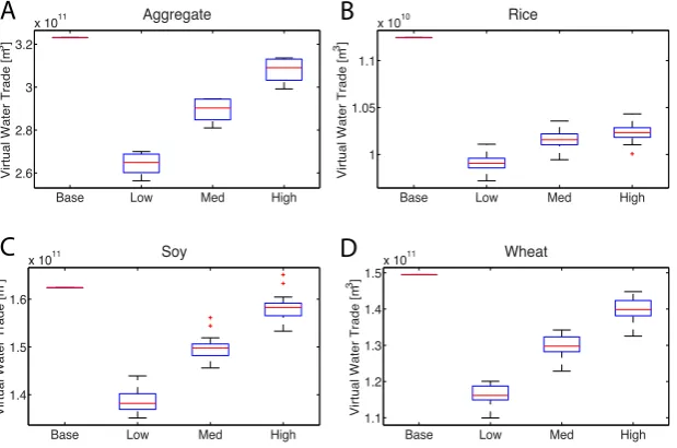
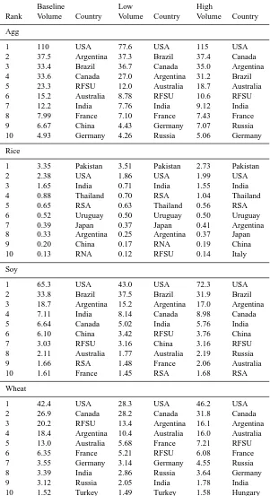
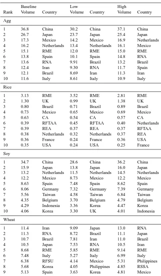
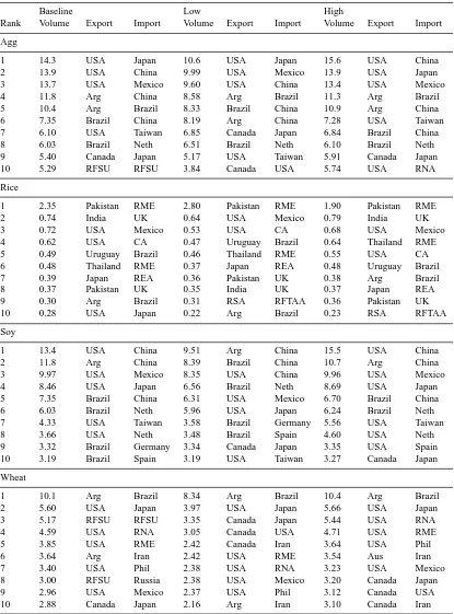
![Fig. 3. Total crop trade [metric tons] and mean VWC [dimensionless] by crop and yield scenario](https://thumb-us.123doks.com/thumbv2/123dok_us/9259683.994859/7.595.134.472.62.278/fig-total-crop-trade-metric-dimensionless-yield-scenario.webp)
Related documents
This involved desk research to identify available training in relation to abuse, neglect and the provision of dignified care; a postal survey of care home managers and
patient management pathway. Occipital Nerve blocks have been shown to be effective and are mandatory for diagnosis but are short acting and Pulsed Radiofrequency may be a
Pennsylvania essay story plot and time in film, Illinois type my research proposal on life sentence for me grand prairie writing a research paper make my term paper on criminal
Understanding culpable wrongdoing requires a conception of
By using social factors, habits and facilitation conditions variables from Triandis’ framework, this paper extends the Technology Acceptance Model (TAM) to derive useful variables
Our results show that the local power of this unit root test is very high under the covariance stationary alternative even for values of the autoregressive parameter very close
explosive behavior in the trend of college tuition and the lack of explosive behavior in the trend of the earnings premium achieved when holding a bachelors degree or higher
The focus of this inquiry concerns the nature of boards and the proposed resources embedded within (board capital). The chapter begins by discussing the research design that
