Computational Modeling and Psvchophysics in Low and Mid Level Vision

(1)

Computational Modeling and Psychophysics in Low- and Mid-Level

Vision

Thesis by Xiaodi Hou

In Partial Fulfillment of the Requirements for the Degree of

Doctor of Philosophy

California Institute of Technology Pasadena, California

2014

(2)

(3)

(4)

Acknowledgements

I would like to express the deepest gratitude to myDoctor-Father, Professor Christof Koch. In my 6-year marathon in the PhD program, Christof has spent great effort guiding me to become a true scientist. With his trust, patience, encouragement, and support, I was able to explore interesting topics as free as Siegfried, from Baltimore harbor to Santa Monica beach, from border-ownership cells to compositional models. Outside the lab, I am greatly indebted to Christof for the sincere help that he offered during the hard times of my life. I also fondly remember our never-ending discussions about tastes of shoe colors, some particular IT company, and the tarantula in Titus Canyon.

Since 2011, I am fortunate enough to be co-supervised by Professor Alan Yuille from UCLA. I enjoyed every single meeting with this British gentleman, to get exposed to his encyclopedic knowledge. More fantastically, Alan has always kept his office door open to me. I would like to thank Alan for his mini math lectures that have greatly helped my research; for his generous financial support during the last quarter of my PhD program; and for every meal he had skipped due to our prolonged discussions.

I am also grateful to other members of my thesis committee, Professor Shinsuke Shimojo and Professor Pietro Perona, who have constantly been providing insightful suggestions for my thesis research.

It is my privilege to have Jonathan Harel, Yin Li, Liwei Wang and Bolei Zhou as my collabo-rators. I would like to thank them for accepting the invitations to my crazy projects, in which we have shared both ecstacies and disappointments. The days we fought back-to-back are invaluable memories to me.

(5)

and Wutu Lin. Like Californian sunshine, they made my stay at Caltech a heartwarming experience. My gratitude also goes to Professor Brian Brophy, for offering me amazing opportunities to the stage play Pasadena Babalon, and the movie PhD Comics; and Professor Ken Pickar, for introducing me to the world of entrepreneurship, which eventually defines my career path.

(6)

Abstract

This thesis addresses a series of topics related to the question of how people find the foreground objects from complex scenes. With both computer vision modeling, as well as psychophysical analyses, we explore the computational principles for low- and mid-level vision.

We first explore the computational methods of generating saliency maps from images and image sequences. We propose an extremely fast algorithm called Image Signature that detects the locations in the image that attract human eye gazes. With a series of experimental validations based on human behavioral data collected from various psychophysical experiments, we conclude that the Image Signature and its spatial-temporal extension, the Phase Discrepancy, are among the most accurate algorithms for saliency detection under various conditions.

In the second part, we bridge the gap between fixation prediction and salient object segmentation with two efforts. First, we propose a new dataset that contains both fixation and object segmentation information. By simultaneously presenting the two types of human data in the same dataset, we are able to analyze their intrinsic connection, as well as understanding the drawbacks of the most popular but inappropriately labeled salient object segmentation dataset. Second, we also propose an algorithm of salient object segmentation. Based on our novel discoveries on the connections of fixation data and salient object segmentation data, our model significantly outperforms all existing models on all 3 datasets with large margins.

(7)

(8)

Introduction

Coming along with the growing amount of image data is the pressing demand for algorithms that analyze these visual information from raw pixels. One aim of computer vision is to inspect an image and present a concise overview of the objects in the scene and their interactions. It requires the visual system to 1) localize the objects in the visual field, and 2) separate the objects from their background content. Known as the figure-ground separation problem, this challenge has been a perennial topic of discussion in computer vision, cognitive science, and neuroscience.

Given an image that contains one or several figures, the raw sensory information has to be perceptually grouped into clusters of foreground regions calledfigures, according to Gestalt psy-chology, and the background calledground. After perceptual organization, the visual information is further passed down to the high-level visual processing stream to fulfill functions such as object detection and face recognition. In computer vision, this process is related to a series of topics such as fixation prediction, salient object detection, and boundary detection. In psychophysics, figure-ground organization is a vital component that connects low-level sensations to high level cognitions. For my doctorate study, I have explored the computational models as well as the psychophysics around the topic of figure-ground separation in natural and synthetic images.

(13)

labels.

There are two types of inconsistencies in the ground-truth of a figure-ground problem: the inter-subject difference, and the intra-inter-subject difference. First, data collected from different inter-subjects may not always come to a consensus. For instance, Fig. 1.1 gives three proposals of the figure segmentation, and each one of them seems plausible. Moreover, different forms of behavioral data capture different aspects of the internal representation. Even though the vision community believes that both eye fixations and hand labels are related to the figure-ground problem, they cannot be used interchangeably due to many differences between these two forms of ground-truths.

Figure 1.1: In one of the lab meetings, Christof showed his new tattoo, which is from Ramon y Cajal’s original drawing of the rodent neocortex. The neocortex tatoo, Christof’s arm, and Christof himself can all be considered as the figure of the image. This example illustrates the ill-defined nature of the figure-ground problem.

1.1 My strategy

(14)

Psychophysical data plays a particular role in our analysis of the figure-ground problem. D-ifferent from today’s common treatments in computer vision (e.g. averaging the data over all subjects), we perform careful analyses of the results of these behavioral experiments. The extra bits of information that we have gained could help us better understand the computational mechanisms of vision system in the following ways:

Defining the problem There are many examples in psychophysics, in which the human visual system fails to parse the information from surprisingly simple patterns. These “counter-examples” of vision provide valuable insights to an algorithm designer. It is critical to understand in what condition, under what kinds of limitation, and with which part of the visual information, humans are able to separate objects from their background in the scene.

Probing the limit of a dataset Like every other experiment, the psychophysical experiment of con-structing the ground-truth of a dataset is noisy. The bias and variance of the ground-truth data determine the limits of benchmarking capability. As the competition among today’s algorithms often goes to 3 digits after the decimal, it is urgent to make sure that the datasets are capable of measuring such tiny difference.

Proposing new directions The ground-truth data can be much more informative than just ranking algorithms based on their benchmark scores. By fully utilizing the rich descriptions from the psychophysical data, we can split the easy and hard sub-problems and propose new directions for future research.

1.2 Thesis Outline

The thesis is composed of several projects that I explored during my graduate study, which can be roughly clustered into the following three topics:

1.2.1 Computational modeling of visual saliency

(15)

of the non-salient background. We formulate the figure-ground separation problem as a signal decomposition problem: x = f +g, wherex is the input image, f is the figure that is spatially

sparse, andgis the ground, which has a sparse representation in the Discrete Cosine Transformed domain (spectrallysparse). Instead of pursuing the exact decomposition ofx, we further show that this decomposition depends implicitly on the binary quantization of the spectral coefficients of the Discrete Cosine Transform ofx. In other words, we can extract, in one line of MATLAB code, a surprisingly simple “bar-code” for each image, and use it to represent the spatial organization of the saliency of the image.

To detect the figures in video clips in Chapter 3, we propose thePhase Discrepancymodel [6], which is a spatial-temporal extension to the original Image Signature. With additional theoretic analysis and experiments on natural image datasets, we show that the Phase Discrepancy model is an effective way of compensating camera self-motion as well as capturing the moving objects. In particular, the algorithm does not rely on prior training on particular features or categories of an image, and can be implemented in 9 lines of MATLAB code.

1.2.2 From fixations to salient objects

Fixation maps are the probabilistic distributions on the image plane. They are often blurry, and do not have clear boundaries of the objects. Therefore, for many computer vision applications, this representation is not as useful as object masks, which not only preserve the location but also the contour of the detected objects. In recent years, a new topic called salient object segmentation is getting the attention from the computer vision community. Despite its goal of attacking the same figure-ground separation problem, the salient object segmentation sub-field is evolved independent-ly from the previous research in fixation prediction. It creates a discomforting segregation of the two research topics.

Another issue is the quality of the ground-truth. Hundreds of algorithms are benchmarked primarily on one dataset with only one labeler to annotate the images. There are no quantitative measures of the quality of such a ground-truth label.

(16)

Second, we also propose an algorithm of salient object segmentation. Based on our novel discoveries on the connections of fixation data and salient object segmentation data, we can ef-fectively make use of the results of existing fixation prediction algorithms. Our model significantly outperformsallexisting models onall3 datasets with large margins.

1.2.3 Psychophysical analyses of boundary labeling and benchmarking

In the third part of the thesis, we discuss topics around the human factors of boundary analysis. Closely related to salient object segmentation, boundary analysis focuses on delimiting the local contours of an object. Defining the boundaries in the image is not an easy task. Previous approaches usually employ many labelers to draw boundaries on every image. Compared with the active re-search on finding a better boundary detector to refresh the performance record, there is surprisingly little discussion on the boundary detection benchmark itself. In Chapter 5, we address the issues in the benchmarking procedure in a popular dataset of boundary detection. The goal of this work [8] is to identify the potential pitfalls during algorithm evaluation. First, with a novel psychophysical experiment, we realize that certain types of human labels, called theorphan labels, are not capable of measuring the performance of today’s algorithms. Second, we discover the issue of precision bubble in the benchmarking procedure that amplifies the effect of the orphan labels. Third, with a series of analyses, we conclude that thestrong boundaries where all human labelers agree is a better-defined sub-problem than “detecting all boundaries in the image.” However, when facing this new challenge, none of today’s major algorithms are capable of detecting such boundaries better than a random method.

(17)

Chapter 2

Saliency Detection using Image

Signature

Abstract

We introduce a simple image descriptor referred to as theImage Signature. We show, within the theoretical framework of sparse signal mixing, that this quantity spatially approximates the fore-ground of an image. We experimentally investigate whether this approximate forefore-ground overlaps with visually conspicuous image locations by developing a saliency algorithm based on the Image Signature.

This saliency algorithm is capable of reproducing the famous search-asymmetry phenomenon on synthetic images. it also accurately predicts human fixation points on many datasets such as the Bruce and Tsotsos [3] benchmark dataset, and does so in much shorter running time. In a related experiment, we demonstrate with a change-blindness dataset that the distance between images induced by the Image Signature is closer to human perceptual distance than can be achieved using other saliency algorithms, pixel-wise or GIST [9] descriptor methods. Finally, we introduce an experiment of face-perspective analysis to further illustrative the perceptual properties that are captured by Image Signature.

2.1 Introduction

The problem of finding all objects in a scene and separating them from the background is known as

(18)

image retrieval, object recognition, and tracking. In this chapter, we provide an approach to the figure-ground separation problem using a binary, holistic image descriptor called the “Image Signa-ture.” It is defined as the sign function of the Discrete Cosine Transform (DCT) of an image. As we shall demonstrate, this simple descriptor preferentially contains information about the foreground of an image – a property that we believe underlies the usefulness of this descriptor for detecting salient image regions.

In Section 2.2, we formulate the figure-ground separation problem in the framework of sparse signal analysis. We prove that the Inverse Discrete Cosine Transform (IDCT) of the Image Sig-nature concentrates the image energy at the locations of a spatially-sparse foreground, relative to a spectrally-sparse background. Then, in Section 2.3, we validate the theoretical limits of Image Signature with a series of experiments on synthetic images.

In Section 2.4, four experiments are presented to quantify the performance of Image Signature in various tasks. First, we use search asymmetry as an illustrative example to show that the Image Signature algorithm faithfully captures the characteristics of human vision behavior. Second, we demonstrate that the saliency maps derived from the Image Signature outperform many leading saliency algorithms on five datasets of eye-movement fixation points. In the same section, we also introduce the reaction-time data collected from nine subjects in a change-blindness experiment. We show that the distance between images induced by the Image Signature most closely matches the perceptual distance between images inferred from these data among competing measures derived from other saliency algorithms, the GIST descriptor, and simpler pixel measures. We conclude the section with a demonstration of the head-orientation-prediction experiment. The binary codes of Image Signature cluster faces with same head orientation with high accuracy, outperforming the best known face orientation detector on the FERET dataset [11].

2.1.1 Related work

Holistic image processing short-circuits the need for segmentation, key-point matching, and other local operations. Bolstered by growing general interest in large-scale image datasets such as 80-million tiny images [12], and ImageNet [13], the early-stage holistic descriptors have become a topic of intense study in computer vision. GIST [9] is an excellent example of such algorithms in this field. Other holistic scene models focus on the separation of foreground and background. For example, Cand`es et al. [14] introduced a sparse matrix factorization model.

(19)

storing only the sign of each DCT component, equivalent to the phase spectrum of a Fourier decomposition. The study of spectral properties of natural images dates back to 1980. In [15] and [16], the authors show that important visual information is stored in the phase spectrum of the image. More recently, statistical models of natural images [17, 18] also argued that natural images have distinctive spectra. Research from computer graphics [19] often categorizes the spectral components of an image as the low-frequency component, i.e. roughly the smoothed copy of the original image, and the high-frequency component, i.e. the residual between the original image and the low-frequency component. Since 2007, saliency detection based on spectral analysis of images has produced amazing, yet not fully-explained results. The first among the family ofspectral saliency

algorithms is Hou’sSpectral Residual. In [20], they used the residual Fourier amplitude spectrum combined with the original phase spectrum to construct the saliency map of an image. This method gives surprisingly good results; however, its original theoretical explanation is flawed. Later studies point out that one can achieve similar saliency maps by discarding the residual amplitude spectrum, and only using the phase information. Since the initial discovery, follow-up studies have made several attempts to explain the computational mechanism of spectral saliency: [21, 22, 23, 24, 25]. In Section 2.3, we will use artificially-generated images to challenge the validity of these alternative theories, and test the necessity and sufficiency of the theory behind Image Signature.

2.2 Image Signature

ˆ

x DCT(x).

sign(x) The entrywise sign operator.

¯

x IDCTsign(ˆx)

, the reconstructed image.

Tx Support set ofx. Ωx Support set ofxˆ.

|x| The absolute value of a real numberx. |S| The cardinality of a setS.

kxk_p The`pnorm of vectorx(p= 2if omitted). hx,yi The inner-product ofxandy.

E(X) The expectation of random variableX. ◦ The Hadamard (entrywise) product operator. ∗ The convolution operator.

(20)

Proposition 1

Proposition 2

Figure 2.1: An illustration of the structure of the proof. Hidden variables are shown in gray boxes. The goal of Image Signature is to represent the spatial support off withx¯. The two propositions can be interpreted as following: Prop. 1 proves that sign(ˆf)can be approximated by sign(ˆx). Prop. 2 proves thatf can be approxmiated by¯f.

We begin by considering gray-scale images that exhibit the following structure:

x=f+b, x,f,b∈RN. (2.1)

frepresents the foreground or figure signal, and is assumed to be sparsely supported in the standard spatial basis. b represents the background, and is assumed to be sparsely supported in the basis of the Discrete Cosine Transform (DCT). In other words, bothf andbˆ have only a small number of non-zero components. Table 2.1 lists the important definitions used throughout the rest of this section.

Performing the exact separation betweenb andf given onlyxand the fact of their sparseness is, in general, very difficult. For the problem of figure-ground separation, we are only interested in the spatial support of f (the set of pixels for which f is non-zero). In this chapter, we show first analytically, then, empirically, that given an image that can be decomposed as Eq. 2.1, we can approximately isolate the support offby taking the sign of the mixture signalxin the transformed domain, and then inversely-transform it back into the spatial domain by computing the reconstructed imagex¯ =IDCTsign(ˆx). Formally, the image signature is defined as:

(21)

If we assume that an image foreground is visually conspicuous relative to its background, then we can form asaliency map m (see [2] for classic use) by smoothing the squared reconstructed image defined above:

m=g∗(¯x◦x¯), (2.3)

wheregis a Gaussian kernel. Our experiments in Section 2.4 show that a simple Gaussian smooth-ing is necessary here, because the supportTf of a salient object is usually not only spatially sparse,

but also localized in a contiguous region.

We also define a distance metricDbetween imagesx1andx2based on the`0distance between image signatures (viz., the Hamming distance):

D(x1,x2) =ksign(xˆ1)−sign(ˆx2)k₀ (2.4)

Building on the idea that the image signature preferentially contains foreground information, this subtraction compares the sparse foreground information in two images without explicitly first com-puting eitherborf. Later, we provide empirical evidence for the utility of this metric.

2.2.1 Image Signature: Foreground Properties

In this section, we provide evidence that, for an image that adheres to a certain mathematical structure, the image signature can be used to approximately obtain the location of the foreground.

Proposition 1 (Signature suppresses background) The image reconstructed from the image sig-nature approximates the location of a sufficiently sparse foreground on a sufficiently sparse

back-ground as follows:

E

h¯f,x¯i

k¯fk · kx¯k

≥0.5, for|Ωb|<

N

6 . (2.5)

Proof 1 Our proof is based on the Uniform Uncertainty Principle (UUP) proposed by Cand`es et al. [26]. LetΘbe a subset of{1,2, . . . , N}of size|Θ|. UUP states that iff is sufficiently spatially sparse, that is, if:

|Tf| ≤α|Θ|/λ , (2.6)

(22)

overwhelm-ing probability, the energy ofˆf supported onΘis bounded:

|Θ|

2Nkfk ≤ kˆf◦1Θk ≤3

|Θ|

2Nkfk, (2.7)

where1Θis the vector with zeros at component indices not inΘand ones at component indices in

Θ.

The over-sampling factor depends on the choice of transform. In [27], Rudelson et al. show

that for Fourier transform,λ=O(log5N). Because of the similarities between DCT and DFT, and

that images are real-valued, this factor is the same for the DCT. In fact, one can construct a signal

x0 ∈R4N from the originalx∈RN as following:

x0_2n=xn x02n−1= 0

x0_4N₋_2n+2 =xN−n+1 x04N−2n+1 = 0,

such that DFT(x)exactly equals DCT(x0).

According to Plancherel’s theorem, we have kfk = kˆf ◦1Ωfk. Then the following inequality can be derived from UUP (Ineq. 2.7):

3|Ωf|

2N kfk ≥ kˆf ◦1Ωfk 3|Ωf|

2N ≥1

|Ωf| ≥ 2

3N . (2.8)

Recall that Ineq. 2.8 holds with overwhelming probability only iff, the foreground is sufficiently

spatially sparse in the sense of Ineq. 2.6.

From this, we estimateh¯f,x¯i:

h¯f,x¯i = IDCT[sign(ˆf)],IDCT[sign(ˆx)] = IDCTsign(ˆf),sign(ˆx)

=

sign(ˆf),sign(ˆx)

= X

i∈Ωb

sign( ˆfi)·sign(ˆxi)

+ X

j /∈Ωb

(23)

Sincef andbare independent from each other, we assume:

P(sign( ˆfi) =sign(ˆbi)|i∈Ωb) = 0.5,

whereP(·)stands for probability. Then:

P(sign( ˆfi) =sign(ˆxi)|i∈Ωb) = P(sign( ˆfi) =sign(ˆbi)|i∈Ωb)

+P(|fˆi|>|ˆbi|,sign( ˆfi)6=sign(ˆbi)|i∈Ωb)≥0.5.

Therefore:

Eh X

i∈Ωb

sign( ˆfi)·sign(ˆxi)

i

≥0. (2.10)

Since sign(ˆbj) = 0, forj /∈Ωb, we have:

X

j /∈Ωb

sign( ˆfj)·sign(ˆxj) =

X

j /∈Ωb

sign( ˆfj)2 ≥ |Ωf| − |Ωb|. (2.11)

Combining Ineq. 2.10, Ineq. 2.11, and Eq. 2.9, we have:

E h¯f,x¯i

k¯fk · kx¯k

≥ _p|Ωf| − |Ωb| |Ωf| · |Ωx|

≥ |Ωf| − |Ωb|

N . (2.12)

Given the bound provided by Ineq. 2.8,

E

h¯f,x¯i

k¯fk · kx¯k

≥ 2

3−

1

N|Ωb| ≥0.5. if we assume that the backgroundbis sufficiently sparse:|Ωb|< N/6.

An important note is that Proposition 1 does not depend on the relative energies of the fore-ground and backfore-ground, kfk and kbk, only their sparseness. This will later be demonstrated empirically in Section 2.3 on synthetic data.

(24)

Proposition 2 For a foreground signalfwith non-zero elements independently drawn from the unit Gaussian distribution, over79%of¯f is expected to be contained in the support of the foreground

Tf. Namely,

E

α

p

α2₊_β2

≥

r

2

π ≈0.7979 where

α =

s X

i∈Tf ¯ f_i2, and

β =

s X

j /∈Tf ¯ f2

j.

Proof 2 First, we quantify the expected correlation betweenˆf and sign(ˆf):

E

ˆf,sign(ˆf)

kˆfk · ksign(ˆf)k

= E

P

ifˆi·sign( ˆfi) kˆfk · ksign(ˆf)k

= E

P

i|fˆi| kˆfk · ksign(ˆf)k

. (2.13)

For zero-mean unit-variance normally distributedfi,

E

_ˆ

f,sign(ˆf)

kˆfk · ksign(ˆf)k

=E(|fˆi|) =

r

2

π . (2.14)

Then, we show that the amount of energy of¯fthat falls intoTf is lower-bounded.

Because the correlation between a pair of signals in the spatial domain is equal to their

corre-lation in the DCT domain, we have:

_ˆ

f,sign(ˆf)

kˆfk · ksign(ˆf)k =

hf,¯fi kfk · k¯fk

= hf,

¯

fi kfkqP

i∈Tf ¯ f_i2+P

j /∈Tf ¯ f_j2

= hf,¯fi

kfkpα2₊_β2 . (2.15)

Let 1Tf be the indicator function that has the value 1 for all elements ofTf and0 elsewhere. From the Cauchy-Schwartz inequality:

(25)

According to Eq. 2.14 and Eq. 2.16:

E

hf,¯fi

kfk · k¯fk

=

r

2

π ≤E

αkfk

kfk ·pα2₊_β2

E_p α

α2₊_β2

≥

r

2

π ≈0.7979. (2.17)

2.2.2 Hamming distance captures the angular difference between structurally

simi-lar images

As we have suggested in Eq. 2.4, the Hamming distanceDbetween two image signatures can be used as a distance metric. We show below how this distance is related to the angular difference between a pair of imagesx1andx2.

Letφi denote theithbasis function of the DCT. We assume thatφi is independent of bothx1 andx2. From [28] (Lemma 2.2), we know that:

Phsign(hx1, φii)6=sign(hx2, φii)

i

= 1

πcos

−1 hx1,x2i kx1_{k · k}_x2_k

.

Letdi(x1,x2)be the indicator function:

di(x1,x2) =







0 if sign(hx1, φii)6=sign(hx2, φii)

1 if sign(hx1, φii) =sign(hx2, φii),

andD(x1,x2) =ksign(ˆx1)−sign(ˆx2)k0=PN_i di(x1,x2), sincehx, φii= ˆxi. Then, the Chernoff bounds guarantee that:

∀ >0, P D >(1 +)N µ

< e−14N µ 2

∀0< <1, P D <(1−)N µ

< e−12N µ 2

,

whereµ = E(di). This result indicates that for large enough N, the following statement is true with high probability:

(1−)D

N ≤

1 πcos

−1 hx1,x2i kx1_{k · k}_x2_k

≤(1 +)D

N . (2.18)

(26)

two images’ structure has changed (for instance, the location of the foreground object has changed), thenD(x1,x2) ≈ 0.5, where no further changes in either foreground or background will push the expectation ofDfurther close to 0.5.

[image:26.595.167.482.197.405.2]

2.3 Image Signature on synthetic images

Figure 2.2: An illustration of the randomly generated images. The first row: f, b, andx in the spatial domain. The second row: The same signals represented in the DCT domain:ˆf,bˆ, andˆx.

In the previous section, we provided theoretical arguments connecting the Image Signature to the spatial support of a sparse foreground. In this section, instead of using natural images, we employ a series of synthetic image experiments. These carefully-constructed cases are the test bed to examine the necessary and sufficient conditions of the algorithm.

Letf,b,x∈_R64×64_{. The support of the foreground is a}₅_×₅_{block (|}_T

f|= 25) that appears at a

random location. The support forbˆis randomly selected in the DCT domain, with|Ωb|= 500. For

i∈ Tf, the amplitude of each pixelfi is drawn from a normal distribution. Similarly, forj ∈Ωb,

eachˆbj is drawn from normal distribution. Fig. 2.2 showsf,b andxin both the spatial and the DCT domains.

The Image Signature reconstruction is illustrated in Fig.2.3. Note that a Gaussian blurring is used to suppress the noise introduced by the sign quantization. Ideally, the standard deviationσof the Gaussian kernel should be proportional to the size of the object of interests. We here choose

(27)

Figure 2.3: An example of the input imagex, the reconstructed imagex¯, and the saliency mapm.

about 10% of the image width).

From Proposition 1, it follows that the reconstructed image x¯ should be insensitive to the amplitude of the foreground. Instead, only its spatial support should be affected. We tested this by multiplying the amplitude of the foreground f by a factor of 10−5, 10−10 and 10−15, while holding the background completely constant. As predicted by the theory, the reconstructed signalx¯

is not changed by the foreground energy until it approaches a minimal numerical value in MATLAB,

2.2×10−16.

Figure 2.4: The reconstructed x¯ with foreground re-weighted as 10−5, 10−10 and 10−15. The saliency maps of these signals remain almost the same despite a huge difference of the foreground amplitude.

The result in Fig. 2.4 directly contradicts the theory of [22], which erroneously explains the spectral saliency as a biologically-plausible process of Gabor linear filtering followed by normal-ization. In fact, the strong invariance to foreground signal strength makes Image Signature immune to today’s rampant and often uncontrolled attempts to impose biological plausibility on any compu-tational model.

(28)

follows a power law (that is, the pixel intensity follows a Pareto distribution). We generated the foreground pixels based on three different distributions – normal distribution, uniform distribution, and Pareto distribution with the PDFf(x) = (1 +x)−2– and tested whether the energy ofx¯ was constrained in the foreground region. For fair comparisons, the foreground was normalized to[0,1]. The proportion (in the sense of Proposition 2) that fell intoTf was: 79.8%,75.6%, and79.3%for

the three distributions, respectively.

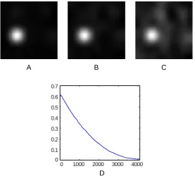
In some scenarios, the background may not be ideally sparse. In Fig. 2.5, we provide an empiri-cal demonstration to test the robustness of this method with respect to non-sparse backgrounds. We observe a clear trend that the energy withinTf drops as the complexity of the background increases.

It is worth mentioning that even with fairly complex backgrounds (with|Ωb|= 3000), the saliency

map still clearly shows the shape of the foreground support of the image.

1000 2000 3000 4000

0 0 0.1 0.2 0.3 0.4 0.5 0.6 0.7

A B C

[image:28.595.187.465.304.554.2]

D

Figure 2.5: Performance of the Signature algorithm with different background complexity on a

64×64image (N = 4096). A.|Ωb| = 1600. B.|Ωb| = 2400. C.|Ωb| = 3200. D. Proportion

of energy concentrated in the foreground supportTf, as a function of background cardinality|Ωb|.

The proportion of energy is the square of the fraction provided in Proposition 2.

(29)

Figure 2.6: Two examples of different frequency components of the background. The first row showsbˆ1,x1, and the saliency mapm1. The second row showsbˆ2,x2, andm2. The two images share the same f. bˆ1 has its support a20×20 rectangle frequency band, whereas the support of

ˆ

b2 is400randomly-selected pixels such thatΩ_b1 = Ω_b2 = 400. Despite different compositions of

their background, the two saliency maps look extremely similar.

Fig. 2.6 is a counter example to any theory that relates spectral saliency to operations on neighboring frequency components. In addition to the original Spectral Residual [20], more recent theories such as [25] revisited the amplitude spectrum and incorrectly concluded that the spikes in the amplitude spectrum determine the foreground-background configuration.

2.4 Experiments

2.4.1 Search asymmetry

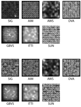
Visual search asymmetry [29] is a well-known phenomenon in which the human performance can be very counter-intuitive. In Fig. 2.7, a subject can easily locate one C in many O’s. However, in the reversed problem of finding the O among C’s, the observer loses her/his ability to detect the figure in the first sight. This striking phenomenon should not be considered as a defect of the cortical algorithm for figure-ground separation. Instead, it reflects some of the “empirical designs” that work for most of the natural scenes.

(30)

SIG AIM AWS DVA

SUN ITTI

GBVS

SUN ITTI

[image:30.595.258.532.85.445.2]

GBVS

Figure 2.7: Visual search asymmetry. There are two scenarios in this visual search task. The easy task is to find the only ‘C’ among numerous ‘O’s, whereas the hard task is to find the unique ‘O’ in ‘C’s. We expect a successful algorithm to detect the easy task but fail in the hard task as humans do. Among all 7 algorithms, Image Signature is the only one that passes this test.

2.4.2 Generating the saliency map of an image

In this section, we report our experimental findings in saliency detection using the Image Signature. As we demonstrated earlier, the reconstructed image detects spatially-sparse signals embedded in spectrally-sparse backgrounds. We will show that the saliency map (Eq. 2.3), which is the Image Signature reconstruction of the foreground spatial support, greatly overlaps with regions of human overt attentional interest, measured as fixation points on the image.

(31)

Input image

Final saliency map

Color channel images

Channel saliency maps

Image

Signature

Figure 2.8: An illustration of the Image Signature algorithm pipeline. The input color image is decomposed into 3 channels. A saliency map is computed for each color channel independently, and the final saliency map is simply the sum across the 3.

from the image reconstructed from the Image Signature:

m=g∗X

i

(¯xi◦¯xi). (2.19)

The standard deviation of the Gaussian blurring kernelgwill be discussed in greater detail in the following section.

(32)

[image:32.595.119.532.116.433.2]

2.4.2.1 Predicting human fixation

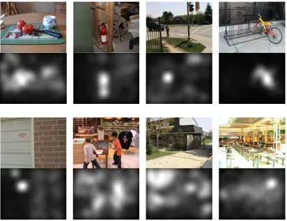
Figure 2.9: Sample images from the Bruce dataset and their corresponding saliency maps using the Image Signature algorithm withσ= 0.05.

To validate the saliency maps generated by our algorithm, we use 5 datasets of human eye-tracking data. One of the first publicly-available datasets is introduced by Bruce and Tsotsos [3] (denotedBruce). It consists of20subjects free-viewing120color images (681×511pixels) for

4 seconds each. Some sample images are shown in Fig. 2.9. The dataset created by Cerf et al. [30] (denotedCerf) is a dataset focusing on human faces. We also used [31] (denoted asJudd), the largest generic dataset of human eye fixations. Moreover, we added the small dataset of [32] (denotedImgSal). Lastly, the new dataset [7] created by us (denotedPASCAL-S) is also used in the evaluation. Background information of the 5 datasets is summarized in Tab. 2.2.

(33)

Name Subject# Image # Year

Bruce 20 120 2006

Cerf 13 200 2008

Judd 15 1003 2009

IS 21 235 2013

[image:33.595.228.423.71.160.2]

PASCAL-S 8 850 2014

Table 2.2: The background information of all 5 datasets used to evaluate algorithms.

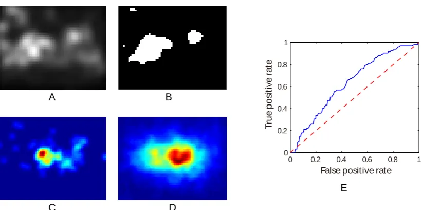
of a saliency algorithm. To remove this center bias, we follow the procedure of [33]: for one image, the positive sample set is composed of the fixation points of all subjects on that image, whereas the negative sample set is composed of the union of all fixation points across all images from the same dataset, except for the positive samples. Each saliency map generated by the algorithm is thresholded and then considered as a binary classifier to separate the positive samples from negative samples. At a particular threshold levelT, the true positive rate is the proportion of the positive samples that fall in the positive (white) region of the binary saliency map (Fig. 2.10-B). The false-positive rate can be computed in a similar way by using the negative sample set. Sweeping over thresholds yields an ROC curve, of which the area beneath provides a good measure of the power of the saliency map to accurately predict where fixations occurred on an image. Chance level is 0.5, and perfect prediction is 1.0.

We compare our saliency maps generated from the Image Signature (denoted SIG) to the following published saliency algorithms: the original Itti-Koch saliency model [2] (denoted Itti), Dynamic Visual Attention model [4] (denoted DVA), Graph-Based Visual Saliency [35] (denoted GBVS), Attention based on Information Maximization [3] (denotedAIM), Adaptive Whitening Saliency [5] (denoted AWS), and Saliency Using Natural image statistic [34] (denotedSUN) for comparison. All of the algorithms are based on the original MATLAB implementations available on the authors’ websites.

An important note about these experiments is that the AUC score is quite sensitive to blurring a saliency map. Some kind of smoothing has been explicitly or implicitly included in most of the algorithms. In order to make a fair comparison, we parameterize the standard deviation of the blurring kernel, and evaluate the performance of an algorithm under different blurring conditions, applied to the final master saliency maps.

(34)

per-E

A B

C D

0 0.2 0.4 0.6 0.8 1

False positive rate

[image:34.595.121.532.76.280.2]

True positive rate

Figure 2.10: An illustration of the AUC computation on the first image in Fig. 2.9. A. The saliency map generated by Lab-Signature algorithm. B. The binary map (thresholded at T = 0.5). C. The positive sample set of human fixations on this image (represented as a heat map). D. The negative sample set of human fixations, containing all fixations across the entire dataset, except those contained in the positive sample set (represented as a heat map). Both Figure C and D are smoothed for display clarity, but the AUC computation uses the exact fixation points. E. The blue curve shows the ROC curve of Image Signature algorithm on this image, with the red reference line indicating the chance level. The area under the blue curve is0.6329.

(35)

0 0.01 0.02 0.03 0.04 0.05 0.06 0.07 0.08 0.62 0.63 0.64 0.65 0.66 0.67 0.68 0.69 0.7 0.71 0.72

AUC Score on BRUCE dataset

Blur Width

(STD of Gaussian kernel in image widths)

AUC Score

(averaged across all images)

0 0.01 0.02 0.03 0.04 0.05 0.06 0.07 0.08 0.64 0.66 0.68 0.7 0.72 0.74 0.76

AUC Score on CERF dataset

Blur Width

AUC Score

0 0.01 0.02 0.03 0.04 0.05 0.06 0.07 0.08 0.6 0.62 0.64 0.66 0.68 0.7 0.72 0.74

AUC Score on IMGSAL dataset

Blur Width

AUC Score

0 0.01 0.02 0.03 0.04 0.05 0.06 0.07 0.08 0.61 0.62 0.63 0.64 0.65 0.66 0.67 0.68 0.69 0.7

AUC Score on JUDD dataset

Blur Width

AUC Score

0 0.01 0.02 0.03 0.04 0.05 0.06 0.07 0.08 0.6 0.61 0.62 0.63 0.64 0.65 0.66 0.67 0.68

AUC Score on PASCAL dataset

Blur Width

AUC Score

[image:35.595.118.530.43.646.2]

AWS AIM SIG DVA GBVS SUN ITTI

(36)

Algorithm AUC Scores

Bruce Cerf Judd ImgSal PASCAL-S

AWS 0.718 0.734 0.691 0.723 0.674

AIM 0.697 0.756 0.687 0.699 0.676

DVA 0.684 0.716 0.659 0.663 0.642

GBVS 0.670 0.706 0.659 0.674 0.655 ITTI 0.656 0.681 0.653 0.668 0.652 SIG 0.710 0.743 0.672 0.699 0.669

SUN 0.665 0.691 0.655 0.664 0.637

Table 2.3: The AUC scores of all 7 algorithms on 5 different fixation datasets.

0 0.2 0.4 0.6 0.8

0.382

0.102 0.131

Average Compute Time (s)

Computational Complexity Comparison

2.060

8.303 9.885

2.517

AWS AIM

SIG DVA

GBVS

SUN ITTI

0.037

Figure 2.12: Average compute time for each algorithm. All algorithms are implemented in the single-thread MATLAB environment on an 8 core 2.5GHz Xeon workstation.

2.4.3 Correlations to change-blindness

Change-blindness [36] is a striking phenomenon in which a subject fails to notice otherwise obvious changes in a pair of images, even when the viewing time extends over a minute or longer. In such an experiment, the original image and a modified version of it alternate repeatedly, but, critically, with a brief masking inserted in between. The ordinary perceptual motion or flicker which would accompany such a change is eliminated by the intervening interval which acts as a sort of mask. The observer must thus rely on his visual memory to identify the change. This is surprisingly difficult.

(37)

demon-Image 1 480 ms

Masking 160 ms

Image 2 480 ms

Masking 160 ms

[image:37.595.220.426.308.509.2]

Image 1 480 ms

...

Figure 2.13: The experimental paradigm for change-blindness. In image 2, the window on the adobe wall has been removed. The subject has to report detection by clicking on the changed area of either image.

strated to be tightly related to the deployment of visual attention. There have been studies [38] that suggest that attended objects are more likely to be encoded in the working memory than non-attended ones.

39.98 s

6.96 s

Figure 2.14: Two sample image pairs. Labels indicate the median reaction time of 9 subjects. Top: the difference is a small white post in the center divider (absent left, present right). Bottom: The difference is the yellow sign on the van (present left, absent right).

(38)

2.4.3.1 Experiment setup

In an experiment conceived by one of the authors (C.K.) and Claudia Wilimizig1,60color images of real world scenes from personal albums were selected. For each original image, 2 modified versions were made, each with one object removed and retouched manually using Adobe Photoshop. The artifacts caused by image processing were kept minimal (Fig. 2.14 gives several examples of the stimuli). During each trial, the original image was displayed for480ms, followed by160msblack masking, and then480msfor the modified image, and then160msmasking. The trial stops after 60s, or when the subject responds by clicking on the image. If the selected location was far away from the true modification, or if the subject did not respond within 60s, or if the response time was less than640ms(before the first onset of the second image), the trial was discarded. 9 naive subjects with normal vision participated in the experiment. Subjects correctly identified the change (or signaled no change) in1011(93.6%) of the9×2×60 = 1080trials.

Because the reaction time distribution among subjects is highly non-linear, we instead compute the log reaction time. The inter-subject correlation (correlating one subject’s reaction time against the remaining 8 subjects) of the reaction times improves from0.3558to0.5305when moving from a linear to a log reaction time, suggesting that the log reaction time correlation is a more meaningful metric than the linear reaction time correlation.

2.4.3.2 Correlate algorithm output with reaction time

As the consequence of a complex cognitive process, the reaction time of a subject in a change-blindness experiment is influenced by many factors. We here correlate such reaction times with various measures derived from the original image and its modified version.

First, reaction times are compared with the saliency of the modified objects. For a good saliency algorithm, we expect the saliency value of an object to be inversely correlated with the reaction time, since the more salient an object is, the more easily a subject can spot it, and thus detect its removal. The saliency value of a removed object is computed by the mean (or sum) pixel intensity of the object region in the saliency map of the original image.

Second, reaction times are compared to the Hamming distance (Eq. 2.4) between the image signature descriptor of the original image and that of the modified image. As described in Sec. 2.2.2, this distance is a sensitive one when images share a background, as they do in the case of

1

(39)

a change-blindness pair. The distance between the descriptors should be related to the extent of difference in their salient, or foreground, regions.

Third, the widely used GIST descriptor [9] is used to describe each image in a change-blindness pair, and reaction times are compared to the GIST distance. [39] showed that perceptually similar images are usually close together in GIST descriptor space. GIST uses 8 orientations, 4 scales for each4×4grid of an RGB color channel, mapping an image to a8×4×16×3 = 1536dimensional real-valued descriptor.

Lastly, we use the pixel-wise distances between the images in the change-blindness pair, and compare these with reaction times. We actually use two pixel-wise measures: the`0and`2distances between the original and modified image. The`0distance is exactly equal to the modified area size. Lethi be the log reaction times of theith subject (a vector with a component for each image in the dataset), andvbe the image pair distances according to one of the methods described above; then, the normalized correlationcis given by correlatingvwith each−hi, normalized by the mean inter-subject correlation, and averaging over 9 subjects:

c= 1 9

9

X

i=1

corr(−hi,v)

Ej6=i

corr(hj,hi)

[image:39.595.122.531.367.639.2]

. (2.20) 0 0.1 0.2 0.3 0.4 0.5 0.6 0.7 0.563 0.368 0.225 0.104 Normalized correlation 0.510 0.404 0.343 0.389 0.387 0.286 AWS AIM SIG DVA GBVS SUN SIG-Hamming ITTI GIST Pixel-L2 Pixel-L0

(40)

The results are summarized in Fig. 2.15. Among all 10 algorithms, the Hamming distance be-tween Image Signature descriptors correlates best with reaction times. That is, among the methods tried here, the perceptual distance between change-blindness pairs is best explained by the image signature descriptor. Given our understanding of the connection between foreground information and the signature, a difficult change-blindness trial is likely one in which the removed object is perceived as part of the background, because in such a trial, we expect a small signature distance.

2.4.4 Image Signature and face orientation

To further illustrate the Image Signature as a compact descriptor of the image, we use the FERET face database [11] as the corpus for analysis. This database contains1400images of200individuals. For each individual, 7 different images were taken, among which, 5 involves head-orientation change (−20◦,−10◦,0◦,10◦,20◦, respectively), and2other images taken in0◦pose contain facial expression and illumination changes. In our experiments, these images are considered as front-face (0◦).

We split the dataset into 700 training images where the labels are readily available for the algorithm, and700testing images where the labels will be estimated using K-NN algorithm. The core idea of this experiment is to illustrate the neighborhood structure of Image Signature defined by Eq.2.4. By choosingK = 20and using majority voting to determine the head orientation for a testing image, this simple algorithm achieved98.86%accuracy. That is, only around 8 images out of700images in the test set were classified as wrong. To the best of our knowledge, the best available result on the FERET database is done by [40] with an accuracy of97%, which means over

20misclassifications.

(41)

SIG

GIST

SIG

GIST

K-NN for identity classification 0 5 10 15 20 400

600 800 1000 1200 1400

Neighborhood size

Wrong label number

Signature GIST 0 5 10 15 20 100

200 300 400 500 600 700 800

Neighborhood size

Wrong label number

Signature GIST

[image:41.595.120.528.175.550.2]

K-NN for perspective classification

(42)

2.5 Conclusion

We introduced the Image Signature as a simple yet powerful descriptor of natural scenes. We proved on the basis of theoretical arguments that this descriptor can be used to approximate the spatial location of a sparse foreground hidden in a spectrally sparse background. We provided synthetic experiments to test the necessity and sufficiency of the assumptions behind Image Signature. We use psychophysical experimental data to show that the approximate foreground location highlighted by the Image Signature was remarkably consistent with both search asymmetry patterns, as well as the locations of human eye-movement fixations, predicting them as good as, or even better than, leading saliency algorithms at a fraction of the computational cost. We provided results from a

(43)

Chapter 3

A Phase Discrepancy Analysis for

Object Motion

Abstract

Detecting moving objects in dynamic backgrounds remains a challenge in computer vision and robotics. This chapter presents a surprisingly-simple algorithm to detect objects in such conditions. Based on theoretic analysis, we show that 1) the displacement of the foreground and the background can be represented by the phase change of Fourier spectra, and 2) the motion of background objects can be extracted byPhase Discrepancyin an efficient and robust way. The algorithm does not rely on prior training on particular features or categories of an image, and can be implemented in 9 lines of MATLAB code.

In addition to the algorithm, we provide a new database for moving-object detection with 20

video clips,11subjects and4785bounding boxes to be used as a public benchmark for algorithm evaluation.

3.1 Introduction

Detecting moving objects in a complex scene is a problem in computer vision of many practical interests. It is closely related to a variety of critical applications such as tracking, video analysis, content retrieval, and robotics. Generally speaking, motion-detection methods can be categorized into the following main approaches: background modeling, view geometry, detection by recogni-tion, and saliency-based detection.

(44)

called background subtraction. The main idea is to learn the appearance model of the background [41] [42]. A moving object in the scene is then detected by subtracting the background image from the current image. However, scene appearance captured by a moving camera, with foreground and backgrounds in arbitrary depths and viewpoints, can be very complicated. Thus, most of the background models perform poorly on moving camera recordings.

To circumvent these problems, some other algorithms detect motion via camera geometry [43] [44]. This approach estimates the camera parameters under certain geometric constraints, uses these parameters to compensate for camera-induced motion, and separate the moving object from the residual motion in the scene [45].

Another branch of popular algorithms stems from object detection, either based on pre-trained detectors, or visual saliency. Some algorithms can detect objects from particular categories, such as faces [46] or pedestrians [47]. These algorithms usually require offline training, and can only handle a very limited number of object categories. Moreover, finding an invariant object detector that overcomes illumination/view-point changes and occlusion is already a challenge in computer vision.

On the other hand, a saliency-based detector relies on the assumption that the object is statisti-cally different from its background. For most of the saliency detection algorithms, unique features of the foreground, such as color, orientation [2], sparse filter responses [4], and temporal cues [48] are utilized to generate a saliency map that predicts the location of an object. The advantage of a saliency-based approach is that it has few assumptions about the appearance of the object, and is therefore capable of detecting unspecified objects without pre-training. Nevertheless, for efficiency considerations, most of today’s models do not incorporate motion cues in an explicit way, which leads to poor performance in video surveillance (as we will see in Section.3.3.4).

In principle, a visual system needs onlymotion cues to detect an moving object – even if the scene is disturbed by camera’s ego-motion. With full knowledge of the optical flow, the mission of object detection is to find the cluster of consistent motion that is induced by the foreground. Nevertheless, the computational burden of an optical flow algorithm is usually very heavy.

3.1.1 Related work

(45)

[image:45.595.172.477.73.321.2]

B)

C)

A)

Figure 3.1: An illustration of moving object detection from a perspective of optical flow analysis. A): A video sequence with both object motions and camera motion. B): The corresponding optical flow.C): The segmentation result that detects the moving objects.

corresponds to a phase change in the Fourier spectrum. For a scene composed ofmobjects, exact recovery is achieved by solving a linear equation with2munknowns. The drawback of this approach is that the number m of objects must be specified beforehand. Moreover, the segmentation and velocity recovery require observing2mframes, which contain every object moving at a constant speed. These constraints preclude Vernon’s approach from real-world applications.

3.1.2 An outline of our approach

We start from a similar perspective to that of Vernon: spatially distributed information can be efficiently accumulated in the Fourier spectrum. However, instead of finding the exact solution for a constrained problem, we seek an approximate solution with a minimal number of assumptions.

(46)

3.2 The Theory

We denotef(x, t)as our observation at timet1_{, where}_x_{= [}_x

1, x2]>is the 2-dimensional vector of a spatial location. LetIbe the ensemble of pixels. For any image, we have the partitionI ={Ft,Bt}. Every pixel belongs to the foregroundF_tor the backgroundB_t.

For typical sampling rates, the ego-motion of the camera is well approximated by a uniform translation of the background. If we know this displacement v = [v1, v2]>, we can predict the appearance of the background in the next frame based on theintensity constancyassumption [50] that the spatial translation does not change pixel values:

f(x, t) =f(x+v, t+ 1), wherex∈ B_t\B_t+1 (3.1) This assumption requires that pixelsxattandx+vatt+ 1belong to the background. We further denoteBˇt= ˆBt+1=BtTBt+1.

Once we have the ground-truth of the ego-motion, we can reconstruct the next frame by shifting every pixel fromxtox+v. This reconstruction is expected to perform poorly for pixels inI −Bˇt, the foreground. Thus, we can take the error as a likelihood function of the appearance of moving objects at certain locations. In other words, the reconstruction error maps(x, t)can be considered as asaliency map[2] for moving objects:

s(x, t) =hf(x+v, t+ 1)−f(x, t)i2. (3.2)

3.2.1 Phase discrepancy and ego-motion

In order to generate the saliency map, we need to know the displacement vectorv. In the Fourier domain, the spatial displacement in Eq. 3.1 can be efficiently represented by the phase of the Fourier spectrum.

LetFx,t(ω) =F[f(x, t)·δxi(x)]denote the 2-D Discrete Fourier transform of a single pixel,

whereω= [ω1, ω2]>, and the indicator functionδxi(x)is defined as:

δxi(x) =







1 ifx∈xi,

0 otherwise.

1

(47)

The Fourier spectrum of the entire imageFt(ω)can be obtained by:

Ft(ω) =

X

xi∈I

Fxi,t(ω)

Known as the translation property [51], a spatial displacement entails a phase change, yet leaves the Fourier amplitudes intact:

Fx+v,t+1(ω) =Fx,t(ω)e−i·Φ(v), (3.3)

where Φ(v) = ω>v = ω1v1 +ω2v2, which we call the Phase Discrepancy in the following discussions.

Because the entire background has approximately the same displacement v, Eq. 3.3 has a compact form forBˇt:

X

xi∈Bˆt+1

Fxi,t+1(ω) =

X

xi∈Bˇt

Fxi,t(ω)e

−i·Φ(v)_. _(3.4)

We have the following decomposition:

Ft+1(ω) =

X

xi∈I

Fxi,t+1(ω) =

X

xi∈Bˇt

Fxi,t(ω)e

−i·Φ(v)₊ X

xi∈I−Bˆt+1

Fxi,t+1(ω)

= Ft(ω)e−i·Φ(v)−

X

xi∈I−Bˇt

Fxi,t(ω)e

−i·Φ(v)₊ X

xi∈I−Bˆt+1

Fxi,t+1(ω).

Although it seems impossible to calculate Φ(v) without the foreground/background partition, in the next section, we show that good approximation of phase discrepancy is achievable in some cases.

3.2.2 Approximating the phase discrepancy

Since it is impossible to quantify the appearance and location of the pixels inI −Bˇt, we assume

Fxi,t(ω)follows an independent normal distribution in the complex domain; that is,

Real{Fxi,t(ω)} ∼N(0,1); Imag{Fxi,t(ω)} ∼N(0,1). (3.5)

For a simpler notation, we define a complex variablezi =Fxi,t(ω). LetZn =

Pn

(48)

sum of this sequence. We have the following:

Real{Zn} ∼ N(0, n) Imag{Zn} ∼ N(0, n)

Because|Zn| =

p

Real{zi}2+Imag{zi}2, it follows aχdistribution with 2 degrees of free-dom:

p(|Zn|=x) = √

nσxe−x2/2. (3.6)

Thus, the expectation of the spectral amplitude is determined by the number of pixels in the summation. More specifically:

E(|Ft(ω)|)

E(| X

xi∈Bˇt

Fxi,t(ω)|)

=

p

#(I)

q

#( ˇB_t)

. (3.7)

The number of pixels in the foreground and background are estimated from our hand labeled database (see Section 3.3). On average, our bounding box of the foreground (an over-estimation of the actual foreground) occupies 5% pixels of the frame 2. Thus, we approximate the phase discrepancy in Eq. 3.5 by:

˜

Φ(v) =∠Ft+1(ω)−∠Ft(ω). (3.8) The estimation error comes from the pixels of the foreground and occluded parts of the back-ground. The cumulative effect of these pixels at frequencyωcan be considered as added noise to variableηto the original variableFt(ω)e−i·Φ(v)in Eq. 3.5, where:

η=− X

xi∈I−Bˇt

Fxi,t(ω)e

−i·Φ(v)₊ X

xi∈I−Bˆt+1

Fxi,t+1(ω).

From Eq. 3.7, we setFt(ω)e−i·Φ(v)to1to determine the distribution ofη:

E(|η|) =

q

2#(I −Bˇt)

q

#( ˇB_t)

≈√0.1; ∠η∼U(0,2π). (3.9)

2

(49)

The upper bound of error inΦ(˜ v)is therefore:

maxΦ(v)−Φ(˜ v)= maxtan−1E(|η|) ≈0.31. (3.10)

Figure 3.2: A diagram of the angular error calculation. GivenE(|η|) =√0.1, the upper bound of the angular error is0.31(17.6◦), and the mean angular error is0.21. (12.3◦)

As long as the approximation in Eq. 3.8 holds, we can construct the estimated spectrumF˜t+1(ω) fromFt(ω)andΦ˜:

˜

Ft+1(ω) = Ft(ω)e−i· ˜

Φ(v)₌_|_F

t(ω)| ·e−i[∠Ft(ω)+ ˜Φ(v)]

= |Ft(ω)| ·e−i[∠Ft+1(ω)]

Finally, the saliency map has the simple form:

s(x, t) =nF−1

Ft+1(ω)

− F−1_˜

Ft+1(ω)

o2

=

n

F−1

|Ft+1(ω)| − |Ft(ω)|

·e−i∠Ft+1(ω)

o2

(3.11)

3.2.3 Eliminating boundary effects

The 2-D Discrete Fourier Transform implicitly implies periodicity of the signal. This property invalidates Eq. 3.1, since pixels around the edge of the frame do not have their correspondences in the next frame. As a result, these frame-edges often have very large reconstruction errors and mislead the saliency maps (see Fig. 3.3.C).

Assume we have two adjacent image frames. We useC₁andC₂ to denote the pixels that lead to boundary effects. As such:

(50)

If we predict frame 2 based on frame 1 (as Eq. 3.11 states), we will have a large error at C1. However, using Eq. 3.11, we have no problem in recovering pixels inC2. Reciprocally, if we reverse the temporal order – reconstructing frame 1 from frame 2 – onlyC2has the boundary effect.

In a more rigid format, we denote the temporally-ordered saliency map that compares the predicted frame 2 with observed frame 2 as−→s(x, t), and the saliency map using reversed sequence (predicting frame 1 from frame 2) as←−s(x, t+ 1). We have:

− →_s₍_x

i, t)> ε, wherexi ∈ C1; ←−s(xi, t+ 1)≤ε, wherexi∈ C1 −

→_s₍_x

i, t)≤ε, wherexi ∈ C2; ←−s(xi, t+ 1)> ε, wherexi∈ C2,

whereεis bounded by Eq. 3.10.

In an elegant form, we finally eliminate the boundary effect by combining the two maps:

s(x, t) =

q

−

→_s₍_x_{, t}₎_{· ←}−_s₍_x_{, t}_{+ 1)} _(3.13)

For∀xi ∈ C1SC2, it is easy to see thats(xi, t)→0as either→−s(xi, t)→0, or←−s(x, t+1)→0. The saliency map generated by Eq. 3.13 is shown in Fig. 3.3-D.

C) D)

[image:50.595.169.479.419.637.2]

A) B)

(51)

3.3 Experiments

3.3.1 Implementing the phase discrepancy algorithm

In MATLAB, the phase discrepancy algorithm is:

FFT1=fft2(Frame1);

FFT2=fft2(Frame2);

Amp1=abs(FFT1);

Amp2=abs(FFT2);

Phase1=angle(FFT1);

Phase2=angle(FFT2);

mMap1=abs(ifft2((Amp2-Amp1).*exp(i*Phase1)));

mMap2=abs(ifft2((Amp2-Amp1).*exp(i*Phase2)));

mMap=mat2gray(mMap1.*mMap2);

Frame1 andFrame2are consecutive frames. In our experiment, the size of image is gray-scaled and shrunk to120×160. On a 2.2GHz Core 2 Duo personal computer, this code performs at refresh rates as high as75frames per second.

One natural way to extend this algorithm to color images is to process each color channel separately, and combine saliency maps for each channel linearly. However, by tripling computa-tional cost, the foreground pixels of color images do not seem to violate the intensity constancy assumption three times stronger than the grayscale image. Indeed, our observation is corroborated by experiments. A comparison experiment of color image detection is in Section.3.3.3. Since our algorithm emphasizes processing speed, we use grayscale images in most of our experiments.

(52)

C) D) B)

[image:52.595.111.535.353.601.2]

A)

Figure 3.4: A comparison of combining the saliency maps of different frames. A): The saliency map computed by 2 frames. B): The saliency map by combining 5 frames (0.25 second). C:) The saliency map by combining 20 frames (1 second).

3.3.2 A new database for moving object detection

There are several public databases for evaluating motion detectors and trackers, such as PETS [52] and CAVIAR [53]. However, very few of them considered camera motion. In this section, we introduce a new database to evaluate the performance of a moving-object-detection algorithm.

Figure 3.5: Sample frames of clips in the database of object-motion detection. Both scenes and moving objects vary from clip to clip.

(53)

the video clip, such as walking pedestrians, cars and bicycles, and sports players. Given the high refresh rate, motion in adjacent frames is very similar. Therefore, it is unnecessary to label every frame. The original 20-FPS videos are given to our subjects for motion detection. For labeling, we asked each subject to draw bounding boxes on a small number of key frames by sub-sampling the sequence on a 0.5-second interval. Eleven naive subjects labeled all moving objects in the video. Some numbers from this database are in Table 3.1.

Items Clips Frames Labelers Key frames Bounding boxes

Number 20 2557 11 297 4785

Table 3.1: A summary of our database.

The evaluation metric of the database is the same as PETS [54]. Although we have data from multiple subjects, the output of an algorithm is compared to one individual at a time. Let RGT denotes the ground truth from the subject. The result generated by the algorithm is denoted asRD. A detection is considered a true positive if:

Area(RGT ∩RD)

Area(RGT ∪RD)

≥T h, (3.14)

The thresholdT hdefines the tolerance of a post-system that is connected to an object detector. If we use a loose criterion (T his small), even a minimal overlap between the generated bounding box and ground-truth is considered a success. However, for many applications, a much higher overlap, equivalent to a much tighter criterion and a larger value ofT h, is needed. In our experiments, we useT h= 0.5.

For the nth clip, using the ith subject as the ground-truth, we useGT_ni, T P_ni, F P_ni to denote the number of ground-truth, true-positive, and false-positive bounding boxes, respectively. The Detection Rate (DR) and False Alarm Rate (FAR) are determined by:

DRn=

P

iT Pni

P

iGTni

F ARn=

P

iF Pni

P

iT Pni +F Pni

. (3.15)

(54)

3.3.3 Performance evaluation

To determine bounding boxes from the saliency map, an algorithm needs to know certain parameters such as spatial scale and sensitivity. To achieve a good performance without being trapped by parameter tuning, we use Non-Maximal Suppression [55] to localize the bounding boxes from the saliency map. This algorithm has three parameters[θ1, θ2, θ3].

First, the algorithm finds all local maxima within a radius θ1. Every local maximum greater thanθ2 is selected as the seed of a bounding box. Then, the saliency map is binarized by threshold

θ3. Finally, the rectangular contour that encompasses the white region surrounding every seed is

considered as a bounding box.

It is straightforward to assume that the parametrization is consistent over different clips in our database, and the locations of objects are independent among different clips. Therefore, we use cross-validation to avoid over-fitting the model. In each iteration, we take 19 clips as the training set to find the parameters that maximize:

X

m∈{training}

DRm(1−F ARm),

And use the remaining clip to test the performance. The final results of DR and FAR are the average among different clips. Samples of detected objects are shown in Fig.3.6. The quantitative result of our model is listed in Table 3.2.

3.3.4 Comparison to other methods