Evaluation of a cosmic ray neutron sensor network for improved land surface model prediction

www.hydrol-earth-syst-sci.net/21/2509/2017/ doi:10.5194/hess-21-2509-2017

© Author(s) 2017. CC Attribution 3.0 License.

Evaluation of a cosmic-ray neutron sensor network

for improved land surface model prediction

Roland Baatz1,2, Harrie-Jan Hendricks Franssen1,2, Xujun Han1,2, Tim Hoar3, Heye Reemt Bogena1, and Harry Vereecken1,2

1_{Agrosphere (IBG-3), Forschungszentrum Jülich GmbH, 52425 Jülich, Germany} 2_{HPSC-TerrSys, 52425 Jülich, Germany}

3_{NCAR Data Assimilation Research Section, Boulder, CO, USA}

Correspondence to:Roland Baatz ([email protected]) Received: 22 August 2016 – Discussion started: 26 August 2016

Revised: 12 April 2017 – Accepted: 19 April 2017 – Published: 16 May 2017

Abstract. In situ soil moisture sensors provide highly ac-curate but very local soil moisture measurements, while re-motely sensed soil moisture is strongly affected by vegetation and surface roughness. In contrast, cosmic-ray neutron sen-sors (CRNSs) allow highly accurate soil moisture estimation on the field scale which could be valuable to improve land surface model predictions. In this study, the potential of a network of CRNSs installed in the 2354 km2Rur catchment (Germany) for estimating soil hydraulic parameters and im-proving soil moisture states was tested. Data measured by the CRNSs were assimilated with the local ensemble transform Kalman filter in the Community Land Model version 4.5. Data of four, eight and nine CRNSs were assimilated for the years 2011 and 2012 (with and without soil hydraulic parameter estimation), followed by a verification year 2013 without data assimilation. This was done using (i) a regional high-resolution soil map, (ii) the FAO soil map and (iii) an erroneous, biased soil map as input information for the sim-ulations. For the regional soil map, soil moisture characteri-zation was only improved in the assimilation period but not in the verification period. For the FAO soil map and the bi-ased soil map, soil moisture predictions improved strongly to a root mean square error of 0.03 cm3cm−3 for the as-similation period and 0.05 cm3cm−3for the evaluation pe-riod. Improvements were limited by the measurement error of CRNSs (0.03 cm3cm−3_{). The positive results obtained}

with data assimilation of nine CRNSs were confirmed by the jackknife experiments with four and eight CRNSs used for assimilation. The results demonstrate that assimilated data of a CRNS network can improve the characterization of soil

moisture content on the catchment scale by updating spatially distributed soil hydraulic parameters of a land surface model.

1 Introduction

large areas but is strongly affected by vegetation and surface roughness (e.g. Temimi et al., 2014). Therefore, in this pa-per an alternative source for soil moisture information is ex-plored which can measure soil moisture more accurately un-der dense vegetation (Bogena et al., 2013). Cosmic-ray neu-tron sensors (CRNSs) measure fast neuneu-tron intensity on an intermediate scale of∼15 ha (Kohli et al., 2015; Zreda et al., 2008), which is the desired application scale of land surface models (Ajami et al., 2014; Chen et al., 2007; Shrestha et al., 2014). Fast neutrons originate from collisions of secondary cosmic particles from outer space with terrestrial atoms. Fast neutrons in turn are moderated most effectively by hydrogen because the mass of a neutron is similar to that of a nucleus of the hydrogen atom. Therefore, the corresponding fast neu-tron intensity measured by CRNSs sneu-trongly depends on the amount of hydrogen within the CRNS footprint, allowing for a continuous non-invasive soil moisture estimate on the field scale. The spatial extent of this measurement is desirable as it matches with the desired grid cell size of a high-resolution land surface model (Crow et al., 2012), and small scale het-erogeneities are averaged over a larger area (Franz et al., 2013; Kohli et al., 2015). Vertical measurement depth ranges from a maximum of ∼70 cm under completely dry condi-tions and decreases to roughly∼12 cm under wet conditions (e.g. 40 vol. % soil moisture) (Kohli et al., 2015; Franz et al., 2012). Worldwide several CRNS networks exist, such as the North American COSMOS network (Zreda et al., 2012), the German CRNS network (Baatz et al., 2014) installed in the context of the TERENO infrastructure measure (Zacharias et al., 2011), the Australian COSMoZ network (Hawdon et al., 2014) and the British COSMOS-UK (Evans et al., 2016).

In this work, fast neutron intensity data measured by CRNSs are assimilated in a land surface model, to evalu-ate the impact those data can have on improving soil mois-ture characterization and land surface model predictions. The ensemble Kalman filtering (EnKF) is one of the most com-monly applied data assimilation methods (Evensen, 1994; Burgers et al., 1998). The EnKF is much less CPU-intensive compared to alternative methods such as the particle filter (e.g. Montzka et al., 2011), because for high-dimensional problems the EnKF requires a much smaller ensemble size to achieve reasonably good predictions. The ensemble Kalman filter (Reichle et al., 2002a; Dunne and Entekhabi, 2005; Crow, 2003; De Lannoy and Reichle, 2016), variants such as the extended Kalman filter (Draper et al., 2009; Reichle et al., 2002b) and the local ensemble transform Kalman fil-ter (Han et al., 2013, 2015) were applied for updating soil moisture states in land surface models. Reichle et al. (2002a) performed a synthetic experiment using L-band microwave observations of the Southern Great Plains Hydrology Exper-iment (Jackson et al., 1999) to analyse the effect of ensemble size and forecast errors. Dunne and Entekhabi (2005) showed that an ensemble Kalman smoother approach, where data from multiple time steps were assimilated to update current and past states, can yield a reduced prediction error compared

to a pure filtering approach. More recently, state updates with the EnKF were tested for the Soil Moisture Ocean Salin-ity (SMOS, Kerr et al., 2012) mission. De Lannoy and Re-ichle (2016) assimilated SMOS temperature brightness and soil moisture retrievals into a land surface model with large improvements in surface soil moisture. However, localized error patterns were not captured well enough, and locally op-timized EnKF error parameters would improve prediction re-sults further.

hydrol-ogy. Montzka et al. (2011, 2013) explored the role of the particle filter for handling non-Gaussianity in soil hydrology data assimilation. They showed that the nonlinear character of the soil moisture retention characteristic is critical for joint state–parameter estimation in data assimilation systems and showed that the particle filter is an interesting alternative for soil hydraulic parameter estimation for 1-D problems. Erdal et al. (2014) investigated the role of bias in the conceptual soil model and explored bias-aware EnKF as a way to deal with it. They argued that the exact location of soil layers is often not known and that this can severely deteriorate the performance of EnKF. Song et al. (2014) worked on a mod-ified iterative EnKF-based filter to handle the non-linearity and non-Gaussianity of data assimilation for the vadose zone. They proposed a modified procedure which avoids the high CPU need of a fully iterative method, but which still gives stable results. Erdal et al. (2015) also focussed on handling of strong non-Gaussianity of the state variable in EnKF under very dry conditions. They showed that classical EnKF fails under such conditions and proposed two alternative strate-gies, both involving transformation of state variables, which also performed favourably under very dry conditions with strongly skewed pressure distributions. All these studies on joint state–parameter estimation showed in general that es-timation of soil hydraulic or land surface parameters im-proves model predictions (strongly), but can be unstable for strongly non-Gaussian distributions and nonlinear problems. For a further literature review on data assimilation in the con-text of hydrological and land surface models, we refer to Re-ichle (2008) and Montzka et al. (2012).

Shuttleworth et al. (2013) developed the Cosmic Ray Soil Moisture Interaction Code (COSMIC), which is a forward operator to be applied for assimilating neutron intensity ob-servations from CRNS. The COSMIC code was evaluated for several sites (Baatz et al., 2014; Rosolem et al., 2014). The COSMIC operator was successfully implemented in the Data Assimilation Research Testbed (Rosolem et al., 2014) to al-low for state updating by the ensemble adjustment Kalman filter (Anderson, 2001). The surface soil moisture informa-tion was propagated into greater soil depth than only the measurement depth using COSMIC in combination with data assimilation (Rosolem et al., 2014). The COSMIC operator was implemented in a python interface that couples the land surface model CLM and the LETKF for joint state–parameter updating (Han et al., 2015). Neutron counts measured by CRNSs have been used in data assimilation studies to up-date model states (Han et al., 2015; Rosolem et al., 2014). Soil hydraulic parameters were also updated by assimilation of neutron counts in one synthetic study (Han et al., 2016), showing its feasibility. CRNSs were also used for inverse es-timation of soil hydraulic parameters of the HYDRUS-1D model (Villarreyes et al., 2014).

This work further explores the value of measured neutron intensity by CRNSs to improve modelling of terrestrial

sys-tems on the catchment scale (Simmer et al., 2015) using a land surface model. The main novelties are as follows:

i. Data from a network of nine CRNSs were assimilated in the CLM with an evaluation of the information gain by this assimilation at the catchment scale. Until now, evaluations with CRNSs were made for a single lo-cation, but not for a complete network of CRNSs. A very important question is whether CRNSs can also im-prove the soil moisture characterization on the catch-ment scale. The high variability of soil moisture at a short distance could potentially limit the CRNS mea-surement value and make updating of soil moisture contents further away from the sensor meaningless. Conversely, soil moisture, soil maps and atmospheric forcings show spatial correlations over larger distances (Kirkpatrick et al., 2014; Korres et al., 2015), which suggests that CRNS measurements potentially carry im-portant information to update soil moisture contents for larger regions (e.g. Han et al., 2012). If it is found that CRNS networks with a density such as that in this study (nine stations per 2354 km2) can improve soil mois-ture content characterization on the catchment scale, this is of high relevance and importance for agricul-tural applications, flood prediction and protection, and regional weather prediction (Whan et al., 2015; Koster et al., 2004; Seneviratne et al., 2010). The main research question addressed in this paper is therefore whether a CRNS network of the density as in this study can im-prove large-scale soil moisture characterization. ii. Soil hydraulic parameters are updated in this study

to-gether with the soil moisture states in a real-world case study. The study in this paper also allows some evalu-ation of the updated large-scale soil hydraulic parame-ters.

2 Materials and methods

2.1 Site description and measurements

Table 1.Site information on elevation (m a.s.l.), average annual precipitation (mm yr−1), CLM plant functional type (Bonan et al., 2002), sand content (%), clay content (%) and the date of the first SWC retrieval assimilated.

Name m a.s.l. Precip. Plant functional type Sand Clay Date of first assimilation

Aachen 232 952 Crops 22 23 13 Jan 2012

Gevenich 108 884 Crops 22 20 7 Jul 2011

Heinsberg 57 814 Crops 18 19 9 Sep 2011

Kall 504 935 C3 grass 20 22 15 Sep 2011

Merzenhausen 94 825 Crops 21 22 19 May 2011

Rollesbroich 515 1307 C3 grass 22 23 19 May 2011

RurAue 102 743 C3 grass 19 26 8 Nov 2011

Wildenrath 76 856 Broadleaf deciduous 65 12 7 May 2012 temperate tree

Wüstebach 605 1401 Needleleaf evergreen 19 23 20 Mar 2011 temperate tree

Figure 1. Map of the Rur catchment and locations of the nine cosmic-ray neutron sensors. The hilly south of the catchment is prone to more rainfall, lower average temperatures and less poten-tial evapotranspiration than the north of the catchment.

in 2011 and 2012 (Baatz et al., 2014). Climate and soil tex-ture of the CRNS sites can be found in Table 1.

The CRNSs were calibrated in the field using gravimet-ric soil samples. At each site, 18 soil samples were taken along 3 circles with distances of 25, 75 and 175 m from the CRNS, and 6 samples were evenly distributed along each cir-cle. Each sample was extracted with a 50.8×300 mm round HUMAX soil corer (Martin Burch AG, Switzerland). The samples were split into 6 sub-samples with 5 cm length each and oven dried at 105◦C for 48 h to measure dry soil bulk density and soil moisture. Lattice water, hydrogen from or-ganic and an-oror-ganic sources, was determined for each site

using a heat conductivity detector (Ray, 1954). Soil bulk density, soil moisture, lattice water and 12 h averaged mea-sured neutron intensity were used to determine calibration parameters specific to each CRNS and the COSMIC opera-tor. This represents a compromise between the measurement noise (which follows a Poisson distribution) and the assumed variation of environmental variables over the averaging time window (Iwema et al., 2015).

2.2 Community Land Model and parameterization The CLM was the land surface model of choice for simulat-ing water and energy exchange between the land surface and the atmosphere (Oleson et al., 2013). Some of the key pro-cesses which are modelled by CLM are radiative transfer in the canopy space, interception of precipitation by the vege-tation and evaporation from intercepted water, water uptake by vegetation and transpiration, soil evaporation, and photo-synthesis, as well as water and energy flow in the subsurface. SWC in CLM is influenced by precipitation, infiltration into the soil, water uptake by vegetation, surface evaporation, and surface and subsurface runoff. To limit the scope and com-plexity of this study, CLM was run using satellite phenology, e.g. prescribed leaf area index data and the biogeochemical module turned off. The biogeochemical module allows CLM to model the vegetation development dynamically, but it re-quires a large spin-up of 1000 years, and little additional gain is expected for this study from these additionally modelled processes.

Vertical water flow in soils is modelled by the 1-D Richards equation. Soil hydraulic parameters are determined from sand and clay content using pedotransfer functions for the mineral soil fraction (Clapp and Hornberger, 1978; Cosby et al., 1984) and organic matter content for the organic soil fraction (Lawrence and Slater, 2008).

param-eter estimates directly dparam-etermine soil hydraulic properties in CLM. The following equations describe how soil texture and organic matter define the soil hydraulic properties in CLM such as porosity, hydraulic conductivity, the empirical ex-ponent B and soil matric potential. Hydraulic conductivity (k(zi), mm s−1) at the depthz between two layers (i and i+1) is a function of soil moisture (θ, m3m−3in layersiand

i+1), saturated hydraulic conductivity (ksat(zi), mm s−1),

saturated soil moisture (θsat, m3m−3) and the empirical

ex-ponentB(Oleson et al., 2013):

k (zi)=

        

φiceksat(zi)

"

(θi+θi+1)

θsat,i+θsat,i+1

#2Bi+3

, 1≤i≤Nlevsoi−1

φiceksat(zi)

θi

θsat,i

2Bi+3

, i=Nlevsoi

,

(1) whereφice is the ice impedance factor. The ice impedance

factor was implemented to simplify an increased tortuos-ity of water flow in a partly frozen pore space. It is calcu-lated withφice=10−Fice using the resistance factor=6

and the frozen fraction of soil porosityFice=θice/θsat,i. Soil

hydraulic properties are calculated separately for the min-eral (min) and organic matter (om) soil components. Total porosityθsat,i is calculated using the fraction of organic

mat-ter (fom,i) with the following:

θsat,i= 1−fom,iθsat,min,i+fom,iθsat,om, (2)

where the organic matter porosity is θsat,om=0.9 and sand

content in percentage (%) determines the mineral soil poros-ityθsat,minas follows:

θsat,min=0.489−0.00126×%sand. (3)

Analogous, the exponentBis calculated with

Bi= 1−fom,iBmin,i+fom,iBom, (4)

whereBom=2.7 is the organic exponent and the mineral

ex-ponent Bmin,i is determined by clay content in percentage

(%) with the following:

Bmin,i=2.91+0.159×%clay. (5)

Saturated hydraulic conductivity is calculated for a con-nected and an unconcon-nected fraction of the grid cell with the following:

ksat(zi)= 1−fpercksat,uncon(zi)+fperc,iksat,om(zi) , (6)

wherefperc,i is the fraction of a grid cell where water flows

with saturated hydraulic conductivity of the organic matter (ksat,om(zi)in mm s−1) through the organic material only, the

so-called connected flow pathway. The saturated hydraulic conductivity of the unconnected part (ksat,uncon(zi), mm s−1)

depends on organic and saturated mineral soil hydraulic con-ductivity:

ksat,uncon= 1−fperc

_1−f

om ksat,min

+fom−fperc

ksat,om

−1

, (7)

where saturated hydraulic conductivity for mineral soil is cal-culated from the grid cell sand content as follows:

ksat,min[zi]=0.0070556×10−0.884+0.0153×%sand. (8)

The fractionfpercis calculated with the following:

fperc=

0.908×(fom−0.5)0.139, fom≥0.5

0, fom<0.5

. (9)

Soil matric potential (mm) is defined as a function of satu-rated soil matric potential (mm) with the following:

ψi=ψsat,i

_θ

i θsat,i

−Bi

=1−fom,iψsat,min,i

+fom,iψsat,om

θi θsat,i

−Bi

, (10)

where saturated organic matter matric potential is

ψsat,om= −10.3 mm and saturated mineral soil matric

potential is calculated from sand content as follows:

ψsat,min,i= −10.0×101.88−0.0131×%sand (11)

2.3 Cosmic-ray forward model

SWC retrievals were calculated from neutron intensity ob-servations with COSMIC (Shuttleworth et al., 2013) fol-lowing calibration results and the procedure of Baatz et al. (2014). COSMIC parameterizes neutron transport within the soil subsurface and was calibrated against the more com-plex Monte Carlo Neutron Particle model MCNPx (Pelowitz, 2005). COSMIC needs considerably less CPU time than the MCNPx model. The code was tested at multiple sites for soil moisture determination (Baatz et al., 2014; Rosolem et al., 2014) and analysed in detail by Rosolem et al. (2014).

COSMIC assumes that a number of high-energy neutrons enter the soil. In the soil, the number of high-energy neutrons is reduced by interactions within the soil, leading to genera-tion of fast neutrons in each soil layer. Before resurfacing, the number of fast neutrons is reduced again by their inter-action with nuclei of elements within soil (Shuttleworth et al., 2013). The number of neutrons,NCRP, that reaches the

CRNS can be summarized in a single integral as follows:

NCRP=NCOSMIC ∞ Z

0

{A(z)[αρS(z)+ρw(z)]

exp

−

ms(z)

L1

+mw(z)

L2

·dz, (12)

where NCOSMIC is an empirical coefficient that is

A(z) is the integrated average attenuation of fast neutrons,

α=0.404−0.101×ρS is the site-specific empirical

coeffi-cient for the creation of fast neutrons by soil,ρS is the dry

soil bulk density (g cm−3), ρw is the total soil water

den-sity (g cm−3), and ms and mw are the masses of soil and

water, respectively, per area (g cm−2)L1=162.0 g cm−2and L2=129.1 g cm−2are scattering lengths for fast neutrons in

solids and water, respectively, that were estimated using the MCNPx code (Shuttleworth et al., 2013). The integrated av-erage attenuation of fast neutronsA(z)can be found numer-ically by solving

A(z)=

2

π

Zπ

0

/2 exp

₋

1 cos(γ )

m_s(z)

L₃ + m_w(z)

L₄

·dγ,

(13) whereγ is the angle along a vertical line below the CRNS detector to the element that contributes to the attenua-tion of fast neutrons, and L3= −31.65+99.29×ρS and L4=3.16 g cm−2are the scattering lengths for fast neutrons

in soil and water, respectively, determined using the MCNPx code (Shuttleworth et al., 2013). The COSMIC operator is discretized into 300 layers of 1 cm thickness up to a depth of 3 m. For each CLM grid cell in the model domain, simulated SWC in all CLM layers is used to generate a weighted SWC retrieval using the COSMIC code. Simulated SWC is handed from the CLM simulation history files to the COSMIC op-erator. Given the vertical SWC distribution of the individual CLM grid cell, COSMIC internally calculates the contribu-tion of each layer to the simulated neutron intensity signal at the soil surface in COSMIC. In this study, the contribution of each CLM soil layer was used to calculate the weighted CLM SWC retrieval corresponding to the vertical distribu-tion of simulated SWC in each grid cell.

Measured neutron intensity of CRNS was used to inversely determine a CRNS SWC retrieval, as by Baatz et al. (2014) assuming a homogeneous vertical SWC distribution. Then, the weighted CLM SWC retrieval is used in the data assimi-lation scheme to relate the CRNS SWC retrieval to the model state. Alternatively, neutron flux data could be assimilated directly within the catchment. This would require calibra-tion data throughout the catchment, which is only feasible using spatially distributed data sets (e.g. Avery et al., 2016). However, high stands of biomass are a major factor for cal-ibration in the Rur catchment (Baatz et al., 2015), and es-timates of biomass come along with high uncertainties. To circumvent the introduction of these additional uncertainties, SWC retrievals are assimilated in this study. Changes in on-site biomass were assumed to be negligible.

2.4 Data assimilation

To further expand the work of Han et al. (2016), this study uses the LETKF (Hunt et al., 2007) to assimilate SWC re-trievals by CRNSs into the land surface model CLM. Up-dates were calculated either for SWC states or jointly for SWC states and soil parameters, depending on the experi-ment setup. For state updates only, the LETKF was used as proposed by Hunt et al. (2007). Calculations were made for an ensemble of model simulations which differed depend-ing on variations in model forcdepend-ings and input parameters. The states of the different ensemble members are indicated byxf

i wherei=1, . . . , N andN is the number of

ensem-ble members; “f” marks the model prediction or forecast be-fore the update. The individual state vectorsxf

i contain the

CLM-simulated SWC of the 10 soil layers and the vertically weighted SWC retrieval obtained with the COSMIC opera-tor. For each grid cell, a matrixXfcan be constructed which contains the deviations of the simulated states with respect to the ensemble meanxf:

Xf= h

xf₁−xf, . . .,xf_N−xf i

. (14)

In the case of joint state–parameter updates, a state aug-mentation approach was followed (Hendricks Franssen and Kinzelbach, 2008; Han et al., 2014). In this case, the aug-mented model state matrixXfis constructed from the simu-lated SWC of the 10 soil layers, weighted SWC, and the grid cell’s sand, clay and organic matter content.

In order to relate the measured neutron intensity with the simulated SWC of CLM, the observation operatorH (COS-MIC) is applied on the measured neutron intensity in order to obtain the expected weighted SWC retrieval at each of the observation locations for each of the stochastic realizations:

yf_i=Hxf_i. (15)

The ensemble realizations of the modelled SWC retrievals at the measurement locationsyf

1 toyfN with respect to the

ensemble meanyfare stored in the matrixYf:

Yf=hyf₁−yf, . . .,yf_N−yfi. (16) The observation error correlation was reduced in space by the factorfredusing the spherical model:

fred=1−(1.5×d/dmax)+

0.5×d/dmax

3

, (17)

whered is the distance to the observation anddmax=40 km

Pa=h(N−1)I+YfTR−1Yfi. (18) In addition, the mean weight vector wa is obtained as fol-lows:

wa=PaYfTR−1y0−yf, (19)

wherey0_{contains the CRNS SWC retrievals at the}

measure-ment locations. In the ensemble space, a perturbation ma-trixWa_{is calculated from the symmetric square root ofP}a_:

Wa=(N−1)Pa1/2. (20)

The final analysisXais obtained from the following:

Xa=xf+Xfwa+Wa. (21)

A more detailed description of the LETKF can be found in Hunt et al., (2007), and details on the implementation of the LETKF in combination with CLM are given by Han et al. (2015).

3 Model and experiment setup 3.1 Model setup

In this study, discretization and parameterization of the hydrological catchment was done on the basis of high-resolution data. The model of the Rur catchment was spa-tially discretized by rectangular grid cells of 0.008◦ size (∼750 m). The model time step was set to hourly. Land cover was assumed to consist of vegetated land units only, and a single plant functional type (PFT) for each grid cell was de-fined. The plant functional types were derived from a re-motely sensed land use map using RapidEye and ASTER data with 15 m resolution (Waldhoff, 2012). Contents of sand, clay and organic matter were derived from the high-resolution regional soil map BK50 (Geologischer Dienst Nordrhein-Westfalen, 2009). Alternative simulations were also performed with the FAO soil map of the global Harmo-nized World Soil Database (FAO, 2012) and with a biased soil texture with a fixed sand content of 80 % and clay con-tent of 10 % (S80 soil map). Average sand and clay concon-tent are 22.5 and 21.4 % for the BK50 soil map and 39 and 22 % for the FAO soil map, respectively. The FAO soil map and the biased soil map represent large error with respect to the soil properties of the BK50 soil map. The FAO soil map and S80 soil map simulations allow the evaluation of the joint state– parameter estimation approach because, given the expected bias, we can evaluate to what extent the soil properties are modified by the data assimilation. This is important because in many regions across the Earth a high-resolution soil map is not available. Land surface models are applied for those re-gions, for example in the context of global simulations, and

hence might be strongly affected by the error in soil proper-ties.

Maximum saturated fraction, a surface parameter which is used for runoff generation, was calculated from a 10 m digi-tal elevation model (scilands GmbH, 2010). Leaf area index data were derived from monthly-averaged Moderate Resolu-tion Imaging Spectrometer data (MODIS). CLM was forced with hourly atmospheric data from the COSMO_DE reanal-ysis data set for the years 2010 to 2013 from the German Weather Service (Deutscher Wetterdienst, DWD). The data were downscaled from a resolution of 2.8 km×2.8 km to the CLM resolution using linear interpolation based on Delau-nay triangulation. Forcing data include precipitation, incident solar and longwave radiation, air temperature, air pressure, wind speed, and relative humidity at the lowest atmospheric level.

3.2 Model ensemble

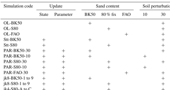
Table 2.Overview of simulation scenarios: open loop (OL-∗) with variation in the soil maps BK50, FAO and S80, data assimilation run with state update (Stt) or joint state and parameter update (PAR) with variation in the soil map perturbation (−10 and−30), and jackknife evaluation runs (jk8-S80-1 to 9, jk8-BK50-1 to 9 and jk4-S80-A to C).

Simulation code Update Sand content Soil perturbation

State Parameter BK50 80 % fix FAO 10 30

OL-BK50 + +

OL-S80 + +

OL-FAO + +

Stt-BK50 + + +

Stt-S80 + + +

PAR-BK50-30 + + + +

PAR-BK50-10 + + + +

PAR-S80-30 + + + +

PAR-S80-10 + + + +

PAR-FAO-30 + + + +

jk8-BK50-1 to 9 + + + +

jk8-S80-1 to 9 + + + +

jk4-S80-A to C + + + +

3.3 Experiment set-up

All simulation experiments in this study used initial condi-tions from a single 5-year spin-up run in which a single forc-ing data set of the year 2010 was repeatedly used as atmo-spheric input. The soil moisture regime became stable after the 5-year spin-up period, and additional spin-up simulations would not affect soil moisture in the consecutive years. Af-ter this 5-year spin-up, soil parameAf-ters and forcing data of the consecutive years were perturbed. From 1 January 2011 onwards, CLM was propagated forward with an ensemble of 95 realizations. On 20 March 2011, the first SWC retrieval was assimilated, and assimilation of SWC retrievals contin-ued until 31 December 2012. In the data assimilation period, soil properties were estimated at every time step when obser-vations were made available. For the year 2013, the model was propagated forward without data assimilation but with an ensemble of 95 realizations. The year 2013 was used ex-clusively as the evaluation period for data assimilation exper-iments.

In total, 31 simulation experiments were carried out using different setups (Table 2). The present setups are intended to cover three different initial soil maps, three different sizes of a CRNS network and two different parameter perturba-tions. Three open loop simulations were run without data as-similation and soil parameter perturbation of 30 % for the BK50 soil map (OL-BK50), the FAO soil map (OL-FAO) and the S80 soil map (OL-S80). These simulations are re-ferred to as reference runs for the respective soil map. Simu-lation results of data assimiSimu-lation runs were compared to the reference runs for quantification of data assimilation bene-fits. Simulations were done with joint state–parameter esti-mation (PAR-∗), two for the BK50 soil map (PAR-BK50-∗), one for the FAO soil map (PAR-FAO-30), and two for the

S80 soil map (PAR-S80-∗). Soil texture was perturbed by 10 or 30 % as indicated by the experiment name (Table 2). Two simulations were done with state updates only for the BK50 soil map (Stt-BK50) and the S80 soil map (Stt-BK50). These 10 simulations form the basic set of experiments.

Besides the data assimilation experiments, a larger num-ber of jackknifing simulations were also conducted to eval-uate the impact of the CRNS data assimilation on SWC at unobserved locations in the model domain. In nine jack-knife experiments, data from eight CRNS locations were as-similated (jk8-∗ simulations) and data of the one remaining CRNSs were not assimilated but kept for evaluation. In ad-dition, three simulations were conducted where data of four CRNSs were assimilated (jk4-∗simulations), and data of the five remaining CRNSs were used for evaluation. These three simulations represent a CRNS network with much less than the existing nine CRNSs. At the evaluation locations, simu-lated SWC (which is affected by the assimilation of the other eight probes) was compared to CRNS SWC retrievals. For jackknife simulations, the perturbation of soil texture was set to 30 %. States and parameters at these sites were jointly up-dated, and simulations were made using either the BK50 or the S80 soil maps as initial parameterization. Therefore, a total of 21 jackknife simulations were performed.

Simulation results were evaluated with the root mean square error (ERMS):

ERMS= v u u u t

n P

t=1

θt,CLM−θt,CRNS2

n , (22)

wheren is the total number of time steps,θt,CLM is SWC

simulated by CLM at time stept andθt,CRNS is the CRNS

the corresponding time step,θt,CLMis SWC prior to

assimi-lation. In case theERMSis estimated at a single point in time

over all CRNSs available, the number of time steps n can be replaced by the number of CRNSs available. The second evaluation measurement in this study is the bias which is, in contrast to theERMS, a measure for systematic deviation:

bias= n P

t=1

θt,CLM−θt,CRNS

n . (23)

4 Results and discussion 4.1 General results

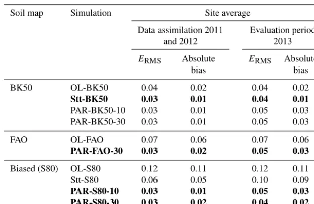
Table 3 summarizes the performance statistics in terms of

ERMS and bias for the assimilation period (2011 and 2012)

and evaluation period (2013). Presented are results for the open loop scenarios with the BK50, FAO and S80, and data assimilation scenarios. Errors of open loop simula-tions were highest for the S80 simulation (0.11 cm3cm−3), followed by the FAO simulation (0.07 cm3cm−3) and the BK50 simulation (0.04 cm3cm−3). Mean absolute bias was highest for the S80 soil map (0.11 cm3cm−3), now as high for the FAO soil map (0.06 cm3cm−3) and lowest for the BK50 soil map (0.02 cm3cm−3). Data assimilation improved simulations more for the S80 soil map (ERMS reduced by

0.08 cm3cm−3) than for the FAO soil map (ERMS reduced

by 0.04 cm3cm−3) or the BK50 soil map (ERMSreduced by

0.01 cm3cm−3_{). The BK50 soil map led to ERMS values}

in open loop simulations lower than 0.05 cm3cm−3_{, which}

left little room for error reduction considering a measure-ment error of 0.03 cm3cm−3. However, slight improvements by 0.01 cm3cm−3 were possible at monitored locations in the data assimilation period but not in the evaluation pe-riod. Joint state–parameter estimation improved simulation results, as shown by the reducedERMSand bias for the S80

and the FAO soil maps. The verification period (2013) with the updated soil hydraulic parameters for the FAO soil map resulted in anERMSvalue of 0.05 cm3cm−3, also clearly an

improvement compared to the open loop run with anERMS

of 0.07 cm3cm−3(Table 3). Joint state–parameter updating resulted in similarERMSvalues for all three initial soil maps:

the BK50, FAO and S80 soil maps (each 0.03 cm3cm3). State updates (Stt-S80) improved ERMS and bias for the

S80 soil map (ERMS=0.06 cm3cm−3 for assimilation

pe-riod) but much less compared to the joint state–parameter updates (PAR-S80-30). TheERMS and bias for simulations

with 10 and 30 % perturbation of soil texture only showed very small differences (smaller than 0.01 cm3cm−3).

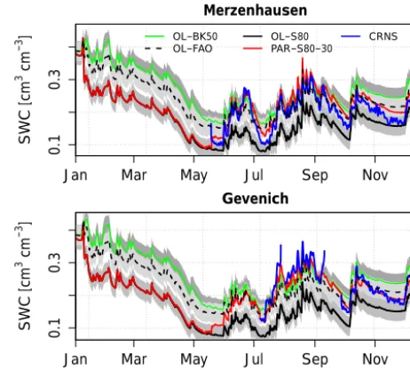
The temporal course of simulated soil moisture in 2011 at the two sites, Merzenhausen and Gevenich, is shown in Fig. 2. The figure illustrates that simulated SWC at both sites

Jan Mar May Jul Sep Nov

0.1

0.3

2011

SWC [cm

3 cm −3 ]

Merzenhausen

OL−BK50

OL−FAO OL−S80PAR−S80−30 CRNS

Jan Mar May Jul Sep Nov

0.1

0.3

2011

SWC [cm

3 cm −3 ]

Gevenich

Figure 2. Temporal evolution of simulated soil water con-tent (SWC) retrievals, calculated with open loop (OL-∗) simulations and data assimilation including parameter updating (PAR-S80-30), together with the CRNS SWC retrieval during the first year of sim-ulation at the sites Merzenhausen and Gevenich. Simulated SWC was vertically weighted using the COSMIC operator to obtain the appropriate SWC corresponding to the CRNS SWC retrieval.

was lowest with the S80 soil map (OL-S80) and highest with the BK50 soil map (OL-BK50), and the FAO soil map re-sulted in intermediate soil moisture (OL-FAO). Mean open loop SWC in 2011 was 0.17 cm3cm−3_{for the S80 soil map,}

0.24 cm3cm−3_{for the FAO soil map and 0.27 cm}3_cm−3_for

the BK50 soil map at both sites. Measurements with CRNS started in May 2011 at Merzenhausen. At Gevenich, the first observation was recorded on 7 July 2011. In the data assimi-lation run shown (PAR-S80-30), modelled SWC was imme-diately affected at both sites, Merzenhausen and Gevenich, as soon as data at Merzenhausen were assimilated. By July, simulated SWC with the biased soil map and data assimi-lation (PAR-S80-30) was already close to the CRNS SWC retrieval at the Gevenich site (Fig. 2). This demonstrates the beneficial impact of data availability for assimilation at one site and the information brought into space by the data as-similation scheme. Figure 2 also shows that the BK50 open loop run was close to the observed SWC at both sites, even without data assimilation.

(PAR-S80-Table 3.Root mean square error (ERMS, cm3cm−3) and mean absolute bias (cm3cm−3) for open loop simulations (OL-∗), data assimilation with state updates (Stt-∗) and joint state–parameter updates (PAR-∗) for both the assimilation period (2011 and 2012) and the evaluation period (2013). Error and bias was averaged over all sites with observations. Site-specific errors and biases are provided in Appendix A1 to A4. The best cases are marked in bold.

Soil map Simulation Site average

Data assimilation 2011 Evaluation period

and 2012 2013

ERMS Absolute ERMS Absolute

bias bias

BK50 OL-BK50 0.04 0.02 0.04 0.02

Stt-BK50 0.03 0.01 0.04 0.01

PAR-BK50-10 0.03 0.01 0.05 0.03

PAR-BK50-30 0.03 0.01 0.05 0.03

FAO OL-FAO 0.07 0.06 0.07 0.06

PAR-FAO-30 0.03 0.02 0.05 0.03

Biased (S80) OL-S80 0.12 0.11 0.12 0.11

Stt-S80 0.06 0.05 0.10 0.09

PAR-S80-10 0.03 0.01 0.05 0.03 PAR-S80-30 0.03 0.02 0.04 0.02

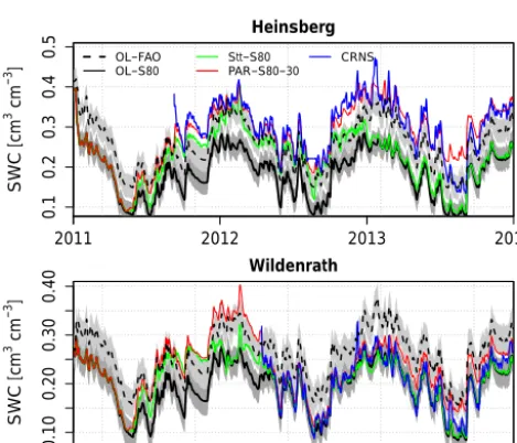
30) than if only states were updated (Stt-S80). This is the case for both the assimilation and the evaluation periods. At the beginning of the evaluation period (first few days of 2013), the Stt-S80 simulation shows an increase in bias between modelled SWC and CRNS. The bias of Stt-S80 re-mained throughout the evaluation period. In contrast, if pa-rameters were previously updated (PAR-S80-30), modelled SWC was close to the CRNS during the evaluation period. Open loop SWC modelled with the FAO soil map is lower than the CRNS SWC retrievals at Heinsberg and higher than CRNS SWC retrievals at Wildenrath. At Wildenrath, results of the OL-S80 run suggest that the initial sand content of the biased soil map is closer to the optimal sand content than the sand content of the FAO soil map. Consequently, the OL-FAO bias was −0.05 and 0.05 cm3cm−3for Heinsberg and Wildenrath, respectively (Tables A1 and A4 in Appendix). At both sites, absolute bias was reduced with joint state– parameter updates to equal or less than 0.01 cm3cm−3(S80 and FAO soil map). The reduced bias is also well reflected in the temporal course of modelled SWC with joint state– parameter updates (PAR-S80-30).

It is interesting to notice that the error values for the ver-ification period are very similar if soil hydraulic parameters were estimated in the assimilation period, independent of the initial soil map (Table 3). ERMS values for the 2013

sim-ulations with state updates only (Stt-BK50 and Stt-BK50) show that in the evaluation period the improvements by state updates (without parameter updates) were small (re-duction by 0.02 and 0.00 cm3cm−3 for S80 and BK50, re-spectively) compared to the improvements obtained by joint state–parameter updates (reduction by 0.07 cm3cm−3 for

S80). This illustrates the benefits of joint state–parameter up-dates compared to state upup-dates only, and that soil moisture states are strongly determined by soil hydraulic parameters. The case of only state updates also illustrates that the im-proved characterization of soil moisture states in the assim-ilation period results in improved initial states for the veri-fication period (Table 3) but in the veriveri-fication period these improvements lose their influence quickly over time (Fig. 3).

4.2 Temporal evolution of meanERMS

Figure 4 shows the temporal evolution of the hourlyERMS

calculated for all nine CRNSs. ERMS was highest for the

S80 open loop run and lowest for the PAR-S80-30 simula-tion. The FAO soil map resulted in errors mostly between 0.05 and 0.1 cm3cm−3, which are lower than the S80 soil map but not as good as simulation results with joint state– parameter updates (PAR-S80-30) or with the BK50 soil map (OL-BK50). State updates did not improve modelled SWC as much as joint state–parameter updates. For most of the time, theERMS of the Stt-S80 run is larger than theERMS of the

OL-BK50 run. During the evaluation period, the open loop run with the FAO soil map (OL-FAO) also performs better than the Stt-S80 run. In contrast, joint state–parameter up-dates to the S80 soil map improved theERMS most of the

simula-Table 4.Root mean square error (ERMS, cm3cm−3) and mean absolute bias (cm3cm−3) for open loop (OL-∗), jackknife simulations with eight CRNSs (simulations jk8-S80-1 to 9 were averaged) and with four CRNSs (simulations jk4-S80-A to C). Results were averaged over the omitted sites only. Data at omitted sites were not assimilated, while at the other sites data were assimilated. At sites where data were assimilated,ERMSand bias were equal to the values found in simulation PAR-S80-30. Site-specific errors and biases are provided in the Appendix A1 to A4. The best cases are marked in bold.

Soil map Simulation Site average

Data assimilation Evaluation period 2011 and 2012 2013

ERMS Absolute ERMS Absolute

bias bias

BK50 OL-BK50 0.04 0.02 0.04 0.02 jk8-BK50-1 to 9 0.06 0.04 0.05 0.04

Biased (S80) OL-S80 0.12 0.11 0.12 0.11 jk8-S80-1 to 9 0.06 0.05 0.06 0.04

jk4-S80-A 0.08 0.06 0.06 0.04

jk4-S80-B 0.06 0.05 0.06 0.05

jk4-S80-C 0.07 0.05 0.07 0.06

2011 2012 2013 2014

0.1

0.2

0.3

0.4

0.5

SWC [cm

3 cm −3 ]

Heinsberg

OL−FAO

OL−S80 Stt−S80PAR−S80−30 CRNS

2011 2012 2013 2014

0.10

0.20

0.30

0.40

SWC [cm

3 cm −3 ]

Wildenrath

Figure 3. Temporal evolution of simulated soil water con-tent (SWC) retrievals, calculated with open loop (OL-∗), data as-similation with state update only (Stt-S80), and data assimila-tion including parameter updating (PAR-S80-30), together with the CRNS SWC retrieval at the sites Heinsberg and Wildenrath for the data assimilation period 2011 and 2012 and the evaluation pe-riod 2013. Simulated SWC was vertically weighted to obtain the appropriate SWC corresponding to the CRNS SWC retrieval.

tion yielded much higherERMSvalues than the BK50 open

loop run.

2011 2012 2013 2014

0.05

0.15

Year

ERMS

[cm

3 cm −3]

OL−BK50

OL−FAO OL−S80PAR−S80−30 Stt−S80

Figure 4.Temporal evolution of root mean square error (ERMS) for hourly SWC retrievals.ERMSis calculated hourly for all nine CRNSs for open loop (OL-∗) runs for soil maps BK50, FAO and S80; joint state–parameter updates (PAR-S80-30); and state updates only (Stt-S80) during the assimilation period with joint state–parameter updates (2011 and 2012) and the verification pe-riod (2013).

4.3 Jackknife simulations

The jackknife simulations investigated the impact of CRNS data on improving simulated SWC at locations beyond the CRNS stations. Spatial improvements are possible by spatial correlation structures of atmospheric forcings, soil hydraulic parameters and soil moisture which are taken into account by the local ensemble transform Kalman filter. The error and bias shown in Table 4 refer to jackknife simulations with the BK50 and the S80 soil map. On average, over the three runs where only data of four CRNSs were assimilated (jk4-S80-∗_{), theE}

RMS was 0.07 m3m−3, which is much lower than

theERMS for the open loop run (0.12 m3m−3) and only a

bit higher than the case where eight CRNSs were assim-ilated (ERMS=0.06 m3m−3 for jk8-S80-∗). The improved

the case of eight assimilated CRNSs. However, for the BK50 soil map whereERMS(0.04 m3m−3) and bias (0.02 m3m−3)

of the open loop run were already good, the jackknife sim-ulations led to slightly higherERMS(0.05 m3m−3) and bias

(0.04 m3m−3). More detailed site statistics (Tables A1 to A4 of the Appendix) demonstrate that all jackknife simulations with the S80 soil map resulted in an improvedERMSat the

omitted locations compared to the open loop simulation, ex-cept for Wildenrath. At sites with large open loopERMS, the

assimilation could reduce theERMSby 50 % or more.

The jackknife simulations illustrate that a network of CRNSs can improve modelled SWC if the soil map informa-tion is not sufficient. This suggests that assimilainforma-tion of CRNS data is particularly useful for regions with little information on subsurface parameters. A trade-off can be expected be-tween the initial uncertainty on soil moisture and parameters, and the density of a CRNS network. In the case of a large un-certainty, like in regions with limited information about soils or a strongly biased soil map (e.g. FAO or S80 soil map) and a low density of meteorological stations, a sparse network of probes can already be helpful for improving soil moisture characterization. The results of the real-world jackknife ex-periments demonstrated that four CRNSs are already benefi-cial, but it is desirable to have more CRNSs for improved pa-rameter estimates. The results also suggest that the additional information gain for an extra CRNS is reduced for a denser network, because the soil moisture characterization did not improve so much more when eight instead of four CRNSs were used for assimilation. However, in regions with a high density of meteorological stations and a high-resolution soil map, it can be expected that a denser CRNS network than that in this study is needed to further lower the error of soil moisture characterization. Further potentially synthetic experiments in other regions with networks of CRNSs are needed to obtain more quantitative information about this. 4.4 Temporal evolution of parameter estimates and

parameter uncertainty

The temporal evolution of sand content estimates during the assimilation period for the nine sites with CRNSs is shown in Fig. 5 for PAR-S80-30, PAR-S80-10, PAR-BK50-30, PAR-BK50-10, jk8-S80-∗ and jk8-BK50-∗. Time series start on 20 March 2011, the date of the first assimilated CRNS SWC retrieval at Wüstebach. At Wüstebach and sites within the influence sphere of Wüstebach (Aachen, Kall and Rollesbroich), sand content estimates were updated from 20 March 2011 onwards. Because of the localization, all other sites show a first update in sand content in May 2012 when Rollesbroich and Merzenhausen start operating, and their data were assimilated. During the data assimilation pe-riod with joint state–parameter updates, all sites show vari-ability in sand content estimates over time with differences in magnitude. Values and spread in sand content estimates amongst the experiments is smaller at the sites

Merzen-hausen, Gevenich, RurAue, Heinsberg and Wildenrath, com-pared to the sites Wüstebach, Aachen and Rollesbroich where spread is considerably larger. At the sites Merzen-hausen, Kall, Gevenich, RurAue and Heinsberg, sand con-tent estimates of the jackknife simulations were close to the sand content of the other data assimilation experiments with joint state–parameter estimation. A comparison of parameter estimates at the end of the assimilation period indicates that initial soil parameterization has a limited effect on the result-ing parameter estimates. Parameter estimates of jk8-BK50-∗ and jk8-S80-∗are close together at the end of the assimilation period.

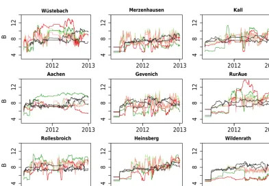
Estimates of the soil hydraulic parameterBand saturated hydraulic conductivity are shown in Figs. 6 and 7 for PAR-S80-30, PAR-S80-10, PAR-BK50-30, PAR-BK50-10, jk8-S80-∗and jk8-BK50-∗. Updates of soil hydraulic parameters start in March and May 2011 with the assimilation of CRNS SWC retrievals, depending on the location. TheBparameter estimates increase for all simulations. Throughout the whole assimilation period the empirical B parameter varies con-siderably within short time intervals. The total range of the

Bparameter estimates is between 2.7 and 14 at all sites. At the sites Merzenhausen, Kall, Aachen, Gevenich and Rolles-broich,Bgenerally ranges between 6 and 10. At Wüstebach, Heinsberg and RurAue, estimates of B range most of the time between 8 and 12, and at Wildenrath, B is below 8. Initial saturated hydraulic conductivity ksat is rather high

(ksat>0.015 mm s−1) in the case of high sand content, i.e. for

the S80 soil map, and rather low (ksat<0.005 mm s−1) in the

case of low sand content, i.e. for the BK50 soil map. In the case of the S80 soil map, at all sites except Wildenrath, high initial ksat estimates decrease quickly through joint state–

parameter updates to values below 0.01 mm s−1_{. The initial}

spread inksatestimates amongst the simulation scenarios

de-creases at most sites. At Wüstebach, Merzenhausen, Aachen, Gevenich, RurAue and Heinsberg, the spread is rather small, particularly at the end of the assimilation period, while at Wildenrathksatranges from 0.005 to 0.015 for individual

ex-periments at the end of the assimilation period.

Temporally unstable parameter estimates imply that there may be multiple or seasonal optimal parameter values. This is also supported by the findings of the temporal behaviour of site-averageERMS(Fig. 4), e.g. during the evaluation

pe-riod when, in the dry summer of 2013, theERMS peaks for

param-2012 2013

10

30

50

70

Sand content [%] BK50

Wüstebach

2012 2013

10

30

50

70

Sand content [%] BK50 Aachen

2012 2013

10

30

50

70

Sand content [%] BK50 Rollesbroich

2012 2013

10

30

50

70

BK50

Merzenhausen

2012 2013

10

30

50

70

BK50

Gevenich

2012 2013

10

30

50

70

BK50

Heinsberg

2012 2013

10

30

50

70

BK50

Kall

2012 2013

10

30

50

70

BK50

RurAue

2012 2013

10

30

50

70

BK50

Wildenrath

Figure 5.At nine sites, estimates of percentage sand content are shown for simulations with parameter update: S80-30 (green), PAR-S80-10 (light green), PAR-BK50-30 (red), PAR-BK50-10 (light red), jk8-S80-∗(black) and jk8-BK50-∗(black). The value of the BK50 soil map is marked at the secondyaxis.

2012 2013

4

8

12

B

Wüstebach

2012 2013

4

8

12

B

Aachen

2012 2013

4

8

12

B

Rollesbroich

2012 2013

4

8

12

Merzenhausen

2012 2013

4

8

12

Gevenich

2012 2013

4

8

12

Heinsberg

2012 2013

4

8

12

Kall

2012 2013

4

8

12

RurAue

2012 2013

4

8

12

Wildenrath

2012 2013

0.005

0.015

k

in

[mm

s

-1]

sat

Wüstebach

2012 2013

0.005

0.015

k

in

[mm

s

-1]

sat

Aachen

2012 2013

0.005

0.015

k

in

[mm

s

-1]

sat

Rollesbroich

2012 2013

0.005

0.015

Merzenhausen

2012 2013

0.005

0.015

Gevenich

2012 2013

0.005

0.015

Heinsberg

2012 2013

0.005

0.015

Kall

2012 2013

0.005

0.015

RurAue

2012 2013

0.005

0.015

Wildenrath

Figure 7.At nine sites, estimates of saturated hydraulic conductivity (top 15 cm) are shown for simulations with parameter update: PAR-S80-30 (green), PAR-S80-10 (light green), PAR-BK50-30 (red), PAR-BK50-10 (light red), jk8-S80-∗(black) and jk8-BK50-∗(black).

eters could give a better parameter-uncertainty characteriza-tion (Shi et al., 2014). Precipitacharacteriza-tion is also an important forc-ing for hydrologic modellforc-ing. For this study, precipitation data from the COSMO_DE re-analysis were used. A product which optimally combines precipitation estimates from radar and gauge measurements is expected to give better precipita-tion estimates than the reanalysis. This could improve the soil moisture characterization and also potentially lead to better parameter estimates. Further improvements and constraining of parameter uncertainty is also possible using multivariate data assimilation with observations such as latent heat flux (e.g. Shi et al., 2014). Also, other error sources related to the model structure play a significant role. These options should be subject to future investigations.

4.5 Latent heat flux

Latent heat flux, or evapotranspiration (ET), is another im-portant diagnostic variable of land surface models (e.g. Best et al., 2015) and is of importance for atmospheric models. Results of the data assimilation experiments showed that soil texture updates altered soil moisture states significantly. In Fig. 8 it is shown that joint state–parameter estimation also altered ET during the evaluation period. Figure 8 shows ET within the evaluation period 2013 across the whole catch-ment for four simulation expericatch-ments. On the one hand, ET was similar for both open loop simulations (S80 and OL-BK50) in the south of the catchment. On the other hand, ET

in the north was up to 80 mm lower per year for the S80 open loop run compared to the BK50 open loop run. The differences can be linked to the drier soil conditions for OL-S80 compared to OL-BK50 simulation results. The differ-ences in ET between the runs with and without parameter up-dates were larger for the S80 soil map than for the BK50 soil map. For PAR-S80-10, ET increased by up to 40 mm yr−1in the northern part of the catchment through data assimilation while the change in ET from OL-BK50 to PAR-BK50-10 is rather small. This is linked to the comparatively larger up-dates made to soil hydraulic parameters.

Figure 8.Annual evapotranspiration (ET) is shown in the year 2013 (evaluation period, no assimilation). This figure demonstrates the impact of parameter updates (PAR-S80-10 and PAR-BK50-10) in comparison to open loop (OL-S80) and the reference soil map (OL-BK50). ET changes in the north but not as much in the south.

the catchment soil parameter uncertainty strongly affects ET. Hence, particularly in the northern part of the catchment, fur-ther observations such as ET measurements are desirable for further improving the land surface model. These additional observations could be used for future land surface model benchmarking (Best et al., 2015) or for more constrained pa-rameter estimates (Shi et al., 2015).

5 Conclusions and outlook

This real-world case study on assimilating CRNS SWC re-trievals into a land surface model shows the potential of CRNS networks to improve subsurface parameterization in regional land surface models, especially if prior information on soil properties is limited. CRNS SWC retrievals were as-similated into the land surface model CLM version 4.5 using the LETKF. SWC and subsurface parameters were updated with the LETKF at unmonitored locations in the catchment considering model and observation uncertainties. Joint state– parameter estimates improved soil moisture estimates during the assimilation and during the evaluation period. The error and bias for the soil moisture characterization was strongly reduced for simulations initialized with a biased soil map and similarly well if initialized with the FAO soil map. Simula-tions initialized with a biased or global soil map approached

similar error statistics with joint state–parameter updates to the ones obtained when the regional soil map was used as input to the simulations. Error values in simulations with the regional soil map were not improved during the evaluation period, because open loop simulation results were already close to the observations. The beneficial results of joint state– parameter updates were confirmed by additional jackknife experiments with eight and four CRNSs for assimilation. In many areas of the world, only global soil maps (e.g. the FAO soil map) are available but there are no detailed high-resolution regional soil maps. This study has shown that in these areas a more advanced subsurface characterization is possible using CRNS measurements and the data assimila-tion framework presented in this study.

op-erator. Both methods require additional field measurements for the verification of vegetation state estimates. The further extension of the data assimilation framework would also en-able the estimation of additional land surface parameters. In addition, the impact of other subsurface parameters, such as subsurface drainage parameters and the surface drainage de-cay factor, on SWC states and radiative surface fluxes has already been shown (Sun et al., 2013). Estimation of these parameters is desirable because of the inherent uncertainty of these globally tuned parameters. However, estimation of soil texture and organic matter content was demonstrated to already be beneficial for improved SWC modelling. Hence, this study represents a way forward towards the integration of CRNS information in the calibration or real-time updating of land surface models.

Appendix A

Table A1.ERMS(cm3cm−3) at CRNS sites for open loop runs and different data assimilation scenarios, for the assimilation period (2011 and 2012). For jackknife experiments (21 in total) only the error of the omitted sites is reported. The best cases are marked in bold.

Soil 2011 and 2012 Rollesbroich Merzenhausen Gevenich Heinsberg Kall RurAue Wüstebach Aachen Wildenrath Average

map ERMS

BK50 OL-BK50 0.058 0.060 0.039 0.039 0.046 0.034 0.056 0.032 0.017 0.042

Stt-BK50 0.031 0.039 0.021 0.021 0.030 0.024 0.039 0.023 0.017 0.027

PAR-BK50-10 0.033 0.036 0.020 0.019 0.032 0.025 0.035 0.045 0.015 0.029

PAR-BK50-30 0.030 0.032 0.018 0.018 0.028 0.024 0.040 0.044 0.016 0.028

jk8-BK50-1 to 9 0.067 0.056 0.065 0.033 0.047 0.051 0.062 0.050 0.091 0.058

FAO OL-FAO 0.097 0.033 0.029 0.056 0.082 0.096 0.079 0.098 0.056 0.070

PAR-FAO-30 0.029 0.033 0.018 0.019 0.028 0.025 0.042 0.056 0.017 0.030

Biased OL-S80 0.169 0.054 0.082 0.119 0.152 0.161 0.110 0.169 0.020 0.115

(S80) Stt-S80 0.098 0.019 0.036 0.050 0.082 0.054 0.083 0.086 0.018 0.058

PAR-S80-10 0.031 0.035 0.023 0.023 0.033 0.024 0.041 0.048 0.015 0.030

PAR-S80-30 0.029 0.032 0.018 0.019 0.028 0.024 0.042 0.068 0.016 0.031

jk8-S80-1 to 9 0.081 0.038 0.060 0.035 0.068 0.043 0.057 0.073 0.095 0.061

jk4-S80-A 0.064 0.038 0.059 0.076 – 0.157 – – – 0.079

jk4-S80-B 0.077 0.041 – 0.051 0.062 0.079 – – – 0.062

jk4-S80-C – 0.073 0.056 – 0.051 – – 0.078 0.109 0.073

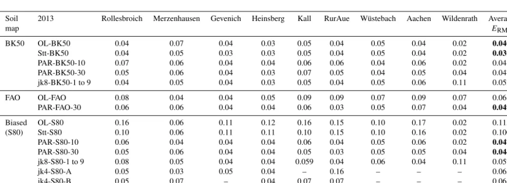
Table A2.ERMS(cm3cm−3) at CRNS sites for open loop, data assimilation and jackknife simulations on the basis of a comparison with CRNS SWC retrievals for the verification period (2013). For jackknife experiments (21 in total) only the error of the omitted sites is reported. The best cases are marked in bold.

Soil 2013 Rollesbroich Merzenhausen Gevenich Heinsberg Kall RurAue Wüstebach Aachen Wildenrath Average

map E_RMS

BK50 OL-BK50 0.04 0.07 0.04 0.03 0.05 0.04 0.05 0.04 0.02 0.040

Stt-BK50 0.04 0.05 0.03 0.03 0.05 0.04 0.05 0.04 0.02 0.039

PAR-BK50-10 0.07 0.06 0.04 0.04 0.06 0.06 0.04 0.06 0.02 0.048

PAR-BK50-30 0.05 0.06 0.04 0.03 0.07 0.05 0.04 0.05 0.04 0.047

jk8-BK50-1 to 9 0.04 0.05 0.04 0.03 0.05 0.04 0.05 0.06 0.11 0.052

FAO OL-FAO 0.08 0.04 0.04 0.05 0.09 0.09 0.07 0.09 0.07 0.068

PAR-FAO-30 0.06 0.06 0.04 0.04 0.06 0.03 0.05 0.07 0.04 0.049

Biased OL-S80 0.16 0.06 0.11 0.12 0.16 0.15 0.10 0.17 0.02 0.115

(S80) Stt-S80 0.10 0.06 0.11 0.11 0.10 0.15 0.10 0.16 0.02 0.100

PAR-S80-10 0.06 0.04 0.04 0.04 0.06 0.04 0.05 0.06 0.02 0.047

PAR-S80-30 0.05 0.06 0.04 0.04 0.05 0.03 0.05 0.05 0.04 0.044

jk8-S80-1 to 9 0.08 0.05 0.04 0.04 0.059 0.04 0.06 0.04 0.11 0.057

jk4-S80-A 0.05 0.03 0.05 0.04 – 0.16 – – – 0.065

jk4-S80-B 0.05 0.07 – 0.04 0.07 0.07 – – – 0.061

Table A3.Bias (cm3cm3) at CRNS sites for open loop, data assimilation and jackknife simulations compared to CRNS SWC retrievals for the data assimilation period (2011 and 2012). For jackknife experiments (21 in total) only the bias of the omitted sites is reported. The best cases are marked in bold.

Soil 2011 and 2012 Rollesbroich Merzenhausen Gevenich Heinsberg Kall RurAue Wüstebach Aachen Wildenrath Mean

map absolute

bias

BK50 OL-BK50 −0.05 0.05 0.02 −0.01 −0.02 −0.01 −0.03 0.00 0.00 0.02

Stt-BK50 −0.02 0.03 0.00 −0.01 −0.01 −0.01 −0.02 0.00 −0.01 0.01

PAR-BK50-10 0.00 0.03 0.00 0.00 0.00 0.00 −0.02 −0.03 0.00 0.01

PAR-BK50-30 −0.02 0.03 0.00 −0.01 −0.01 −0.01 −0.03 −0.03 0.00 0.01

jk8-BK50-1 to 9 −0.05 0.05 0.05 −0.01 0.00 −0.04 −0.04 −0.04 0.09 0.04

FAO OL-FAO −0.09 0.02 −0.01 −0.05 −0.07 −0.09 −0.06 −0.09 0.05 0.06

PAR-FAO-30 −0.01 0.03 0.00 −0.01 −0.01 −0.01 −0.03 −0.04 0.01 0.02

Biased OL-S80 −0.17 −0.05 −0.08 −0.12 −0.15 −0.16 −0.09 −0.17 −0.01 0.11

(S80) Stt-S80 −0.09 0.00 −0.03 −0.04 −0.07 −0.04 −0.07 −0.07 −0.01 0.05

PAR-S80-10 0.00 0.03 0.00 −0.01 0.00 0.00 −0.03 −0.04 0.00 0.01

PAR-S80-30 −0.02 0.03 0.00 −0.01 −0.01 −0.01 −0.03 −0.06 0.00 0.02

jk8-S80-1 to 9 −0.07 0.02 0.05 −0.01 −0.06 −0.03 −0.03 −0.07 0.09 0.05

jk4-S80-A −0.05 −0.02 −0.03 −0.06 − −0.16 − − − 0.06

jk4-S80-B −0.07 0.02 − −0.04 −0.05 −0.07 – – – 0.05

jk4-S80-C – 0.04 0.02 – −0.02 – – −0.07 0.11 0.05

Table A4.Bias (cm3cm−3) at CRNS sites for open loop, data assimilation and jackknife simulations compared to CRNS SWC retrievals for the data assimilation period (2011 and 2012). For jackknife experiments (21 in total) only the bias of the omitted sites is reported. The best cases are marked in bold.

Soil 2013 Rollesbroich Merzenhausen Gevenich Heinsberg Kall RurAue Wüstebach Aachen Wildenrath Mean

map absolute

bias

BK50 OL-BK50 −0.03 0.06 0.01 0.00 −0.02 0.00 −0.02 0.01 0.00 0.02

Stt-BK50 −0.01 0.04 0.00 0.00 −0.01 −0.01 −0.02 0.00 −0.01 0.01

PAR-BK50-10 0.06 0.05 0.01 0.02 0.04 0.04 0.02 −0.04 0.00 0.03

PAR-BK50-30 0.03 0.05 0.00 0.02 0.04 0.03 −0.01 −0.03 0.03 0.03

jk8-BK50-1 to 9 −0.02 0.04 0.01 −0.01 −0.03 −0.02 −0.04 −0.05 0.11 0.04

FAO OL-FAO −0.08 0.02 −0.02 −0.04 −0.08 −0.08 −0.05 −0.08 0.06 0.06

PAR-FAO-30 0.04 0.05 0.00 0.02 0.03 0.00 −0.02 −0.06 0.03 0.03

Biased OL−S80 −0.15 −0.05 −0.10 −0.11 −0.16 −0.15 −0.09 −0.16 −0.01 0.11

(S80) Stt-S80 −0.09 −0.05 −0.10 −0.10 −0.08 −0.14 −0.09 −0.15 −0.01 0.09

PAR-S80-10 0.04 0.03 −0.03 0.03 0.05 0.03 0.03 −0.04 −0.01 0.03

PAR-S80-30 0.03 0.05 −0.01 0.02 0.03 0.01 −0.01 −0.03 0.03 0.02

jk8-S80-1 to 9 −0.07 0.03 0.02 0.02 −0.05 −0.02 −0.04 −0.03 0.10 0.04

jk4-S80-A 0.00 0.01 0.03 −0.03 − −0.15 − − − 0.04

jk4-S80-B −0.03 0.06 − −0.03 −0.06 −0.06 − − − 0.05

Competing interests. The authors declare that they have no conflict of interest.

Acknowledgements. The authors gratefully acknowledge the support by the SFB-TR32 “Pattern in Soil–Vegetation–Atmosphere Systems: Monitoring, Modelling and Data Assimilation”, funded by the Deutsche Forschungsgemeinschaft (DFG), and TERENO (Terrestrial Environmental Observatories), funded by the Helmholtz-Gemeinschaft. The authors also gratefully acknowledge the computing time granted by the John von Neumann Institute for Computing (NIC) and provided on the supercomputer JURECA at Jülich Supercomputing Centre (JSC). Finally, the authors acknowl-edge and thank four anonymous referees for providing constructive comments and the Editor, Nunzio Romano, for guiding the revision process.

The article processing charges for this open-access publication were covered by a Research

Centre of the Helmholtz Association.

Edited by: N. Romano

Reviewed by: four anonymous referees

References

Ajami, H., McCabe, M. F., Evans, J. P., and Stisen, S.: Assessing the impact of model spin-up on surface water-groundwater interac-tions using an integrated hydrologic model, Water Resour. Res., 50, 2636–2656, doi:10.1002/2013wr014258, 2014.

Anderson, J. L.: An ensemble adjustment Kalman filter for data assimilation, Mon. Weather Rev., 129, 2884–2903, doi:10.1175/1520-0493(2001)129<2884:Aeakff>2.0.Co;2, 2001.

Avery, W. A., Finkenbiner, C., Franz, T. E., Wang, T. J., Nguy-Robertson, A. L., Suyker, A., Arkebauer, T., and Munoz-Arriola, F.: Incorporation of globally available datasets into the rov-ing cosmic-ray neutron probe method for estimatrov-ing field-scale soil water content, Hydrol. Earth Syst. Sci., 20, 3859–3872, doi:10.5194/hess-20-3859-2016, 2016.

Baatz, R., Bogena, H. R., Hendricks Franssen, H. J., Huisman, J. A., Qu, W., Montzka, C., and Vereecken, H.: Calibration of a catchment scale cosmic-ray probe network: A comparison of three parameterization methods, J. Hydrol., 516, 231–244, doi:10.1016/j.jhydrol.2014.02.026, 2014.

Baatz, R., Bogena, H. R., Hendricks Franssen, H. J., Huis-man, J. A., Montzka, C., and Vereecken, H.: An empirical vegetation correction for soil water content quantification us-ing cosmic ray probes, Water Resour. Res., 51, 2030–2046, doi:10.1002/2014WR016443, 2015.

Bateni, S. M. and Entekhabi, D.: Surface heat flux estima-tion with the ensemble Kalman smoother: Joint estimaestima-tion of state and parameters, Water Resour. Res., 48, W08521, doi:10.1029/2011wr011542, 2012.

Best, M. J., Abramowitz, G., Johnson, H. R., Pitman, A. J., Bal-samo, G., Boone, A., Cuntz, M., Decharme, B., Dirmeyer, P. A., Dong, J., Ek, M., Guo, Z., Haverd, V., Van den Hurk, B. J. J., Nearing, G. S., Pak, B., Peters-Lidard, C., Santanello, J. A.,

Stevens, L., and Vuichard, N.: The Plumbing of Land Surface Models: Benchmarking Model Performance, J. Hydrometeorol., 16, 1425–1442, doi:10.1175/Jhm-D-14-0158.1, 2015.

Bogena, H. R., Herbst, M., Hake, J. F., Kunkel, R., Montzka, C., Pütz, T., Vereecken, H., and Wendland, F.: MOSYRUR – Water balance analysis in the Rur basin, in: Schriften des Forschungszentrums Jülich, Reihe Umwelt/Environment, Forschungszentrum Jülich, Jülich, 2005.

Bogena, H. R., Huisman, J. A., Baatz, R., Hendricks-Franssen, H. J., and Vereecken, H.: Accuracy of the cosmic-ray soil water content probe in humid forest ecosystems: The worst case scenario, Wa-ter Resour. Res., 49, 5778–5791, doi:10.1002/wrcr.20463, 2013. Bonan, G. B., Levis, S., Kergoat, L., and Oleson, K. W.: Land-scapes as patches of plant functional types: An integrating con-cept for climate and ecosystem models, Global Biogeochem. Cy., 16, 1021, doi:10.1029/2000GB001360, 2002.

Brutsaert, W.: Hydrology: an introduction, Cambridge University Press, Cambridge, New York, 605 pp., 2005.

Burgers, G., van Leeuwen, P. J., and Evensen, G.: Analysis scheme in the ensemble Kalman filter, Mon. Weather Rev., 126, 1719– 1724, doi:10.1175/1520-0493(1998)126<1719:Asitek>2.0.Co;2, 1998.

Chen, F., Manning, K. W., LeMone, M. A., Trier, S. B., Alfieri, J. G., Roberts, R., Tewari, M., Niyogi, D., Horst, T. W., Oncley, S. P., Basara, J. B., and Blanken, P. D.: Description and eval-uation of the characteristics of the NCAR high-resolution land data assimilation system, J. Appl. Meteorol. Clim., 46, 694–713, doi:10.1175/Jam2463.1, 2007.

Chen, Y. and Zhang, D. X.: Data assimilation for transient flow in geologic formations via ensemble Kalman filter, Adv. Water Resour., 29, 1107–1122, doi:10.1016/j.advwatres.2005.09.007, 2006.

Clapp, R. B. and Hornberger, G. M.: Empirical Equations for Some Soil Hydraulic-Properties, Water Resour. Res., 14, 601– 604, doi:10.1029/Wr014i004p00601, 1978.

Cosby, B. J., Hornberger, G. M., Clapp, R. B., and Ginn, T. R.: A Statistical Exploration of the Relationships of Soil-Moisture Characteristics to the Physical-Properties of Soils, Water Resour. Res., 20, 682–690, doi:10.1029/Wr020i006p00682, 1984. Crow, W. T.: Correcting land surface model predictions for the

im-pact of temporally sparse rainfall rate measurements using an en-semble Kalman filter and surface brightness temperature obser-vations, J. Hydrometeorol., 4, 960–973, 2003.

Crow, W. T., Berg, A. A., Cosh, M. H., Loew, A., Mohanty, B. P., Panciera, R., de Rosnay, P., Ryu, D., and Walker, J. P.: Upscaling Sparse Ground-Based Soil Moisture Observations for the Valida-tion of Coarse-ResoluValida-tion Satellite Soil Moisture Products, Rev. Geophys., 50, Rg2002, doi:10.1029/2011rg000372, 2012. De Lannoy, G. J. M. and Reichle, R. H.: Assimilation of

SMOS brightness temperatures or soil moisture retrievals into a land surface model, Hydrol. Earth Syst. Sci., 20, 4895–4911, doi:10.5194/hess-20-4895-2016, 2016.