To Forbear or not to Forbear? A Behavioral Perspective of Multimarket Competition

(1)

ScholarWorks @ Georgia State University

Chemistry Theses Department of Chemistry

4-20-2010

An Analysis of Prominent Water Models by Molecular Dynamics

Simulations

Quentin Ramon Johnson

Georgia State University, [email protected]

Follow this and additional works at: https://scholarworks.gsu.edu/chemistry_theses

Recommended Citation Recommended Citation

Johnson, Quentin Ramon, "An Analysis of Prominent Water Models by Molecular Dynamics Simulations." Thesis, Georgia State University, 2010.

https://scholarworks.gsu.edu/chemistry_theses/30

This Thesis is brought to you for free and open access by the Department of Chemistry at ScholarWorks @ Georgia State University. It has been accepted for inclusion in Chemistry Theses by an authorized administrator of

(2)

BY MOLECULAR DYNAIMCS SIMULATIONS

by

QUENTIN JOHNSON

Under the Direction of Dr. Donald Hamelberg

ABSTRACT

Water is the most common solvent for most biological reactions, therefore it is vital that

we fully understand water and all its properties. The complex hydrogen bonding network that

water forms can influence protein-protein and protein-substrate interactions and can slow protein

conformational shifts. Here, I examine an important property of water known as energetic

roughness. The network of interactions between individual water molecules affect the energy

landscape of proteins by altering the underlying energetic roughness. I have attributed this

roughness to the making and breaking of hydrogen bonds as the network of hydrogen bonds

constantly adopts new conformations. Through a novel computational approach I have analyzed

five prominent water models and have determined their inherent roughness to be between 0.43

and 0.62 kcal/mol.

INDEX WORDS: Abstract, Thesis, Energetic Roughness, Department of Chemistry, Quentin

(3)

AN ANALYSIS OF THE ENERGETIC ROUGHNESS OF PROMINENT WATER MODELS

by

QUENTIN JOHNSON

A Thesis Submitted in Partial Fulfillment of the Requirements for the Degree of

Master of Science

in the College of Arts and Sciences

Georgia State University

(4)

Copyright by

Quentin Johnson

(5)

AN ANALYSIS OF THE ENERGETIC ROUGHNESS OF PROMINENT WATER MODELS

by

QUENTIN JOHNSON

Committee Chair: Donald Hamelberg

Committee: Donald Hamelberg

Stuart Allison

Davon Kennedy

Electronic Version Approved

Office of Graduate Studies

College of Arts and Sciences

Georgia State University

(6)

DEDICATION

I would like to take this opportunity to dedicate this manuscript to Dr. Donald

Hamelberg, who introduced me to the field of computational chemistry and has been a constant

inspiration for me. Dr. Hamelberg has not only been my advisor throughout this process but has

(7)

ACKNOWLEDGMENTS

I am very appreciative for the boundless friendship, advisement and acceptance that I

have incurred throughout my stay here at Georgia State University. I would like to thank Dr.

Donald Hamelberg for the direction he has given me and all the help he has afforded me over the

years. Also, a thank you goes to Adam Velasquez for his friendship and pressure lifting attitude

that helped me make it through the hard days. Urmi Doshi deserves my thanks for the help she

gave me and also for her stern but constructive criticism. I would also like to thank Jennifer

Kelley for providing assistance and experience in the lab. Thank you Yao Xin for being a soft

spoken leader in the lab giving me an idea of how to roll with the punches. Thank you to Lauren

McGowan for giving me someone to identify with in the lab and providing a few laughs in times

of need.

I would also like to extend my thanks to Dr. Alfons Baumstark for his excellent

advisement, for working hard to help me achieve this goal and for introducing me to Dr.

Hamelberg. Thank you to Will Lovett for his help every semester and for making sure that I

graduated. A special thank you goes to the entire department for helping me get to this point and

for accepting me into the fold.

I would like to thank my mother Sylvia Johnson, sister Monique Johnson, and father

George Johnson for believing in me and providing support throughout my college career. I can

always count on my family to make a vacation a vacation. I appreciate all the holidays I spent

with you all and am only sorry that in my pursuit of education I have not had more time for the

(8)

TABLE OF CONTENTS

ACKNOWLEDGEMENTS ... iv

LIST OF TABLES ...viii

LIST OF EQUATIONS...ix

LIST OF FIGURES ...x

LIST OF ABBREVIATIONS……….………xi

1 INTRODUCTION ...1

1.1 Purpose of the Study...1

1.2 Expected Results ...1

1.3 Molecular Dynamics Background...1

1.4 Energetic Roughness Background...3

1.5 Water Roughness...5

1.6 Slaving...5

1.7 Importance of Study...7

2 RESULTS...8

3 DISCUSSION...15

3 CONCLUSION...18

4 EXPERIMENTAL ...20

4.1 TIP3P...20

4.2 TIP4P...27

4.3 SPC/E...28

4.4 TIP5P...29

(9)

4.5 Vacuum...31

(10)

LIST OF TABLES

(11)

LIST OF EQUATIONS

Equation 1.1...2

Equation 1.2...3

Equation 1.3...6

Equation 2.1...9

Equation 2.2...10

Equation 2.3...10

Equation 2.4...10

(12)

LIST OF FIGURES

Figure 1.1...6

Figure 1.2...8

Figure 2.1...9

Figure 2.2...11

Figure 2.3...12

Figure 2.4………..13

Figure 3.1...16

(13)

LIST OF ABBREVEATIONS

fs femto seconds

ns nano seconds

ps pico second

MD molecular dynamics

(14)

CHAPTER 1

INTRODUCTION

Purpose of Study

Water plays a very important role in the dynamics and function of proteins, and the

network of interactions between individual water molecules affects the energy landscape of

proteins by altering the underlying energetic roughness. The purpose of this study is to

mathematically evaluate the amount that water contributes to this “roughness” in hopes to better

understand the functions of proteins and assess the differences of the water models.

Expected Results

I expect that the effect of the interactions of water on the overall energy landscape by

alteration of the energetic roughness will be substantial considering that that hydrogen bond

network of water is intricate and vast. The energetic component of hydrogen bond network

rearrangements has been estimated to be between 0.8 and 1.5 kcal/mol using x-ray absorption

spectroscopy. This value represents the average thermal energy required to distort a hydrogen

bond or to rearrange or change the fully coordinated configuration of water to a configuration

with a broken hydrogen bond to the donor. I expect that the contribution of water's energetic

roughness will fall somewhere in this range, approximately 1 kcal/mol.

Molecular Dynamics Background

Molecular dynamics (MD) is a type of computer simulation that combines chemistry,

math and physics to simulate the motions and interactions of atoms, molecules, and

biomolecules. Atoms and molecules are set up to interact for a period of time by approximations

(15)

is frequently utilized in the study of proteins and other biomolecules. It is possible to take

snapshots of crystal structures and probe features of the motion of molecules through nuclear

magnetic resonance NMR, however no conventional experiment allows access to all the time

scales of motion with atomic resolution. Molecular dynamics normally employs crystal structure

from the Protein Data Bank or PDB as the starting structures of a multitude of biomolecules and

adds velocities and coordinates through a combination of complex algorithms, physical

chemistry and physics. Molecular dynamics allows scientists to visualize the motions of

individual atoms in a way that is not possible in laboratory experiments. Molecular dynamics is

based on statistical mechanics and uses a potential energy function with multiple components to

define a system as well as the time-dependent behavior of the system.

E = Ebondstretch + Eangle-bend + Edihedral + Eother + Enonbonded

(16)

(Equation 1.2: Amber force field function-Note that despite the term force field, this

equation defines the potential energy of the system; the force is the derivative of this

potential with respect to position.)

The MD method relies on the assumption that statistical ensemble averages are equal to time

averages of the system. This assumption is known as the Ergodic hypothesis. MD simulations

are usually done over short time scales, pico to nano seconds, because longer simulations require

extreme computational power and can be very computationally expensive.

Energetic Roughness Background

While the concept is relatively abstract, it is a physical anomaly and can be defined

through mathematic means. Energetic roughness results in the slowing of bimolecular motion by

restricting the biomolecule through bumps in the energy landscape, during conformational

transitions for example. Somewhat like speed bumps in a road slowing a car from moving from

(17)

sub-cellular processes. However, switching between different ensembles of protein

conformations that are important for function can result in complex dynamics due to the

complexity of the energy landscape . The energy landscape of proteins is very rugged and

represents a huge number of conformational states, including the surrounding water molecules

that are an integral part of biomolecular structure . The unevenness of the energy landscape could

lead to kinetic traps if it is comparable or much greater than kBT, where kB is the Boltzmann

constant and T is the temperature. Theories have been developed to highlight the nature of the

inherent roughness of the energy landscape of biomolecules, and experiments have been

proposed and carried out to measure this property . The ruggedness of the energy landscape is

due mainly to intra-protein, protein-water, and water-water interactions that are formed and

broken in different substates or as the protein undergo large conformational changes between

two different substates. Characterizing the nature of the underlying landscape roughness and

calculating the magnitude of the different contributions will provide a better insight into the

dynamics and function of proteins.

Here, we have calculated the effect of water on the energy landscape of proteins using

molecular dynamics simulations and by developing a model based on the position space analog

of the Ornstein-Uhlenbeck process to extract the contribution of the energetic roughness. This

approach has allowed us to study an important property of the widely used atomistic simulation

water models that directly affects the dynamics of biomolecular systems. When the roughness,

which is calculated to be around ~1 kcal/mol, is much greater than kBT, the network of hydrogen

bonds could increase the frustration on the landscape of proteins. Also, this aspect of protein

dynamics could have much broader implications on the function of some classes of enzymes as

(18)

Water Roughness

In addition to the ruggedness of energy landscape of protein, water also has a rugged

potential energy landscape, with each point representing a different hydrogen bonding network.

Therefore, water by itself has slow dynamics, since it has to form and break hydrogen bonds as

the network of hydrogen bonds rearranges . The energetic component of hydrogen bond network

rearrangements has been estimated to be between 0.8 and 1.5 kcal/mol using x-ray absorption

spectroscopy. This value represents the average thermal energy required to distort a hydrogen

bond or to rearrange or change the fully coordinated configuration of water to a configuration

with a broken hydrogen bond to the donor. However, the exact structure of liquid water and the

average thermal energy associated with hydrogen bond rearrangements are still unresolved and

controversial. The quality of the data and the interpretation of the results have been questioned.

Nonetheless, forming and breaking of the hydrogen bonds of water molecules around proteins

will undoubtedly have an effect on the dynamics of proteins that will show up as an energetic

component on the overall protein energy landscape. This process can lead to slaving of

biomolecules by the solvent.

Slaving

Protein motions can be slaves to explicit solvent fluctuations. Basically, a surrounding

solvent of a protein controls the rate of motion/folding. Frauenfelder and coworkers postulate

that protein folding has the same temperature dependence as the α-fluctuations in the bulk

solvent but is much slower. Large-scale protein motions follow the solvent fluctuations with

rate coefficient kα but can be slower by a large factor. Slowing occurs because large-scale

(19)

(Equation 1.3: Slaving equation. 'Frauenfelder')

(Figure 1.1: A schematic description of protein folding. 'Frauenfelder')

In Figure 1.1 the real space representation of protein folding, the unfolded polypeptide (U) folds

into the working protein (N). In conformational space, the protein makes a random walk through

the high-dimensional energy landscape. (a) A 1D cross-section through the energy landscape

showing the U (blue), TSE (red), and N (green) conformational basins. The long arrow

represents a folding path with an overall rate k f, whereas the short arrow shows a single step,

with a rate k α, in the conformational diffusion during folding. (b) A 2D cross-section through

(20)

from a U conformation, proteins make a Brownian walk in the conformational space until they

finally fall into the ensemble of N substates.

Importance of Study

The role of water on protein dynamics has been studies extensively . As proteins undergo

constant thermal motions, they also displace the surrounding water molecules as they change

conformational states. The effect of the viscosity of the aqueous medium on the motions of

proteins is manifested, at the microscopic level, by water molecules that form a dynamic network

of hydrogen bonds. This network of hydrogen bonds constantly rearranges as proteins move

from one conformational state to another. Breaking and reforming of these hydrogen bonds

contribute to the roughness on the overall energy landscape of the protein and could enslave the

motion of proteins, especially at low temperature. The magnitude of the roughness due to

hydration on the energy landscape is not well characterized. A full understanding of this aspect

of protein dynamics has much broader implications, such as the dynamic effects of de-solvated

molecules relative to that of solvated molecules, the low temperature behavior of solvated

biomolecules, and the fundamental nature of water hydrogen bond network.

In order to quantitatively capture the energetic effect of water on the landscape of

proteins, we have developed a model and presented a novel approach to tease out the extent to

which the (energetic) roughness of water influences the energy landscape and the dynamics of

proteins. We carried out a series of molecular dynamics simulations using Ace-Ala-Pro-Nme

(Figure 1) at different temperatures in four widely used explicit simulation water models (TIP3P,

SPC/E, TIP4P-EW, and TIP5P) using the pmemd module in the AMBER 10 suite of programs

and the modified version of the Cornell et al force field. The Langevin thermostat was used to

regulate the temperature, with a collision frequency of 10 ps-1 and the particle mesh Ewald

(21)

the set temperature and a constant pressure of 1 bar in a periodic cubic box with the edges of the

box at least 10 Å away from the peptide. The simulation was then carried out for 10 ns at

constant temperature and volume (NVT ensemble) using an integration time step of 2fs and

applying the SHAKE algorithm to all bonds involving hydrogen.

(Figure 1.2: Depicts the Ace-Ala-Pro-Nme, shows the omega angle used in dihedral data. Also gives a plot of ω versus time.)

CHAPTER 2

RESULTS

[image:21.612.77.460.237.370.2]

The dynamics of the ω-bond angle (CA-C-N’-CA’) of Ace-Ala-Pro-Nme, shown in

Figure 1.2, were monitored during the course of the simulation. If the velocity autocorrelation

function along the ω-bond angle has a much shorter characteristic timescale compared to that of

the displacement of ω, which is the case for biomolecular dynamics in general, we can use the

diffusive motion of ω on an effective one dimensional energy profile, U(ω), to describe the

actual complicated motion of the peptide along that degree of freedom. The diffusive motion of

the peptide on this effective 1D energy profile is generally described by the Smoluchowski

(22)

( )

( ) ( )

⎥ ⎦ ⎤ ⎢ ⎣ ⎡ ∂ ∂ + ∂ ∂ ∂ ∂ = ∂ ∂ ω ω ω ω ω ω ω U T k t p t p D t t p B , , ,

(Equation 2.1: Smoluchowki equation)

where p(ω,t) is the time-dependent probability distribution of the peptide ω-bond angle, and the

diffusion coefficient D is assumed to be independent of ω. The probability distribution of the ω

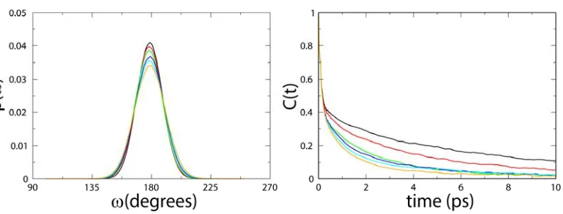
[image:22.612.83.479.312.463.2]

-bond angle in the energy basin of the trans configuration is approximately Gaussian, as shown in

Figure 2.1.

(Figure 2.1: The distribution of the peptide ω bond between Ala and Pro in Ace-Ala-Pro-Nme at six different temperatures (275, 300, 325, 350, 375, and 400 K) for SPC/E.)

Therefore, the effective 1D potential landscape, U(ω), of the motion of the peptide along the ω

-bond angle in the trans basin is approximately described by a harmonic potential where C is the

effective spring constant and γ≈ 180o

(

)

2

2 )

(ω = C ω−γ

U

(23)

Furthermore, the Brownian motion in a harmonic potential described as a position space analog

of the Ornstein-Uhlenbeck (OU) process has been studied extensively, and the autocorrelation

function of ω is given by

) exp( ) ( ) 0

( t >=< 2 > −tDC k_BT

<ω ω ω

(Equation 2.3: autocorrelation function)

where

C T k_B

>= <ω2

(Equation 2.4)

The autocorrelation functions of ω at six different temperatures (275, 300, 325, 350, 375, and

400 K) calculated from the simulation data in the SPC/E water model are also shown in Figure

1.3. Fitting the tail of the autocorrelation functions in Figure 1.3 using Equations 1.6 and 1.7 to a

single exponential, we obtained D, the diffusion coefficient, of the displacement of the ω-bond

angle on the effective 1D harmonic well at different temperatures.

Previously, Zwanzig showed by analytically solving the Smoluchowski equation

(Equation1.4) that the diffusion coefficient, D, on an effective 1D landscape is related to the

underlying energetic roughness, ε, by Equation 2.5.

] ) (

exp[ ε k T θ D

D= ₀ − _B

(Equation 2.5)

Where D0 is the diffusion coefficient on the smooth potential energy surface. Subsequently, it

was shown that for a protein system in an effective 1D energy profile θ = 2 , and the quadratic

(24)

distribution. If the energetic roughness is θ = 1, then the roughness is uniform and evenly

distributed.

From the diffusion coefficients, D, derived from fitting the autocorrelation function to an OU

process at different temperatures, we obtain a plot of equation 2.5, as shown in Figure 2.2 for the

simulations in the different water models, and also in vacuum.

(25)

The data fits very well when θ = 2. We further confirmed that θ = 2 is a better fit than θ = 1 by

[image:25.612.90.509.207.626.2]

increasing the temperature range and carrying out simulations in TIP4P-EW at 600 K. From

Figure 2.4, we calculated the roughness for the different water models and vacuum (the baseline)

as shown in Figure 2.3.

Water model Roughness,

ε (kcal/mol)

Self-diffusion coefficient (x 10-5 cm2/s)

at ~25oC and 1 atm

Structure of water model (A ball and stick model with partial charges on each charge center)

Vacuum 0.45 -

TIP3P 0.87 5.06 _5.65

SPC/E 1.01 2.49 _2.76

TIP4P-Ew 1.00 2.4

TIP5P 1.08 2.62

Experimental - 2.23

2.3

(Table 2.1 and Figure 2.3: Table of raw energetic roughness of vacuum, TIP3P, TIP4P. SPC/E,

(26)

If one considers the roughness of Ace-Ala-Pro-Nme in vacuum as the baseline, then TIP5P

contribute ~0.63 kcal/mol of additional roughness to the energy landscape. TIP4P-EW and

SPC/E contribute about ~0.56 kcal/mol. The roughness contributed by TIP3P (~0.42 kcal/mol) is

the smallest. Therefore, SPC/E, TIP4P-EW, and TIP5P are slightly “rougher” than TIP3P. It is

also important to note that the self diffusion coefficient of TIP3P is about twice that of SPC/E,

TIP4P-EW, and TIP5P, and the difference in energetic roughness could be partly attributed to

that as well.

(27)

While Figure 2.4 is not a completely true to life representation of the energetic landscape of the

peptide used in this experiment, it is useful in illustrating the difference that adding water to a

system causes in the overall energetic landscape. The roughness of water are manifested as the

bumps in the landscape where proteins must scale these hills to reach the next conformational

(28)

CHAPTER 3

DISCUSSION

The question still remains, what is the main contributing factor to the energetic roughness

of water? By looking at the partial charges on the water models with three charged centers

(SPC/E, TIP3P, and TIP4P-EW), one could see that the absolute magnitude of the partial charges

is larger in SPC/E and TIP4P-EW than in TIP3P, and the increase correlates with a slight

increase in the energetic roughness. This observation therefore raised the possibility that majority

of the contribution to the energetic roughness is due to hydrogen bonding, which is electrostatic

in nature in the classical definition of the water models. Alternatively, one could argue that the

roughness may have artificial component due to the Langevin thermostat and the random noise

associated with it. However, it is important to note that the roughness is distinctly different for

the different water models under similar conditions and using the same thermostat. Nonetheless,

in order to test the effect of the Langevin thermostat on the energetic roughness, we have

doubled the collision frequency to 20/ps and repeated the simulation for TIP4P-EW water as

shown in Figure 3.1 (magenta). We clearly see that overall the dynamics is slightly slower, as

expected at higher friction, but the slope of the line and hence the roughness is almost identical

to simulations with a smaller collision frequency (Figure 3.1, red line). Changing the collision

(29)

(Figure 3.1: Plot of equation 2.5 for TIP4P with collision frequency 10/ps and 20/ps, TIP4P with

no charges, and vacuum)

Consequently, I have hypothesized that the main source of the energetic roughness is due to the

forming and breaking of hydrogen bonding interactions between the water molecules, since the

other non-bonded van der Waals interactions are far weaker. As noted above, the description of

the hydrogen bonding interaction in the current classical model is purely electrostatic.

Therefore, in order to test this hypothesis, we have repeated the simulation of the peptide in a

(30)

molecules, thus eliminating the electrostatic interactions between the water molecules. The

simulations were carried out with the same box sizes as those of the simulations with full partial

charges at the different temperatures, in order to only capture the effect of eliminating the

electrostatic interactions. For this model system of TIP4P-EW water with no partial charges, the

energetic roughness is reduced considerably, as shown in Figure 3.1 (orange). We clearly see

that by eliminating the partial charges on the water molecules, the slope of the line and hence the

roughness also decreases considerably and is now comparable to that in vacuum. However, the

data for TIP4P-EW with zero partial charges fits Equation 2.5 better with θ = 1 than with θ = 2,

implying that without the electrostatic interactions the roughness is more uniform and evenly

distributed. This change in the nature of the roughness could be attributed to the fact that van der

Waals interactions are very short ranged and are due only to the oxygen, since the radius of

hydrogen for these water models is zero. On the other hand, electrostatic interactions are

longer-ranged, and a slight change could have implications far away, adding to the randomness of this

interaction.

Using this approach, we have calculated the contribution to the roughness of proteins by

the most widely used water models for atomistic simulations of biomolecules. This approach has

allowed us to study one property of the solvent that directly affects the dynamics of biomolecular

systems. It also presents a very important and an additional property of water that can be taken

into account when optimizing simulation water models, if need be, to reproduce experimental

results and its effects on protein dynamics. The network of hydrogen bonds formed by water

molecules around proteins (as depicted in Figure 3.2) that is constantly rearranging as the protein

changes conformation manifests itself as roughness on the underlying energy surface. The water

molecules immediately around the peptide form transient, cage-like structure that is held together

(31)

hydrogen bonds break and re-form to alter the network of hydrogen bonds. Each arrangement of

the network of water molecules is an energetic substate of the water that provides the additional

roughness on the energy landscape of proteins.

(Figure 3.2: Depiction of Pro-Nme with the first shell of hydration enclosing

(32)

Conclusion

The energetic roughness could have several implications for protein chemistry and

motions. For example, when θ = 2 in equation 3, the effect of the roughness on the dynamics of

the protein will become very pronounced at low temperature and will enslave the motions of

proteins. At higher temperature, when the roughness is much less than kBT, the effect of water

molecules on the dynamics will be predominately due to the internal frictional drag of the

molecules and less on the roughness of water, since the energetic roughness is ~1 kcal/mol

Additionally, proteins that function as enzymes usually provide an environment in a

cavity or binding site that is usually devoid of any appreciable amount of solvent. Taking away

the specific interactions of the active site of proteins, the effect on the catalytic process of

moving the substrate from the aqueous medium to the active site is still not fully understood.

From the above results, it could be suggested that the change in environment of the substrate

would change the frictional drag and the topological features of the energy landscape of the

protein substrate or other ligand that is not limited to the reduction of the energetic roughness

and thus “paving” the surface along the reactions coordinate for the conformational transition to

occur. This change in the topology of the landscape would most likely manifest itself by altering

the kinetic prefactor, in addition to the dominate effect due to transition state stabilization or

(33)

CHAPTER 4

EXPERIMENTAL

TIP3P

We carried out a series of molecular dynamics simulations using Ace-Ala-Pro-Nme at

different temperatures using the pmemd module in the AMBER 10 suite of programs and the

modified version of the Cornell et al force field. The Langevin thermostat was used to regulate

the temperature, with a collision frequency of 10 ps-1 and the particle mesh Ewald method was

used to treat long-ranged electrostatic interactions. The system was equilibrated at the set

temperature and a constant pressure of 1 bar in a periodic cubic box with the edges of the box at

least 10 Å away from the peptide. The simulation was then carried out for 10 ns at constant

temperature and volume (NVT ensemble) using an integration time step of 2fs and applying the

SHAKE algorithm to all bonds involving hydrogen. The system was first created using the xleap

program by first constructing the Ace-Ala-Pro-Nme peptide. Next the peptide was solvated

using the TIP3P water model from the xleap library. Xleap was then utilized to generate a

topology file and an initial coordinate file. The topology and coordinate files were then

combined with a minimization input file in the Amber10 program in the minimization step.

This minimization step is used to bring the system to a global energy minimum while keeping

the system in a periodic box. The minimization was carried out for 0.01 ns. A total of eighteen

minimizations were done in sets of three for six different temperatures ( 275K, 300K, 325K,

350K, 375K, 400K).

-Minimization parameters: The minimization was carried out under the following

(34)

imin- set to 1, so that a minimization will be performed

ntx-set to 1, so that X is read formatted with no initial velocity information.

npr- set to 10, so that every 10 steps energy information was printed in the output file.

ntwv- set to 0, so that all velocity output was inhibited.

ibelly- set to 0, so that no subset of atoms was allowed to move.

ntmin- set to 1, so that for NCYC cycles the steepest descent method is used then

conjugate gradient is switched on.

nstlim- set to 10000, so that 10000 steps are performed.

nscm- set to 0, so that the position of the center-of-mass of the molecule is not reset.

dt- set to 0.001, so that each step takes 0.001 fs.

tempi- set to 100K, however this parameter is ignored due to this being a minimization

temp0- set to target temp, so that the minimization is carried out at this average

temperature

ig- set to 71277, 11297, or 61267 depending on the run, this parameter affects the set

of pseudo-random values used for Langevin dynamics. It was set to a different

value for three seperate run in order to produce some variation in data for error

sake.

ntp- set to 1, so that pressure is kept constant

ntb- set to 2, so that pressure is kept constant

comp- set to 44.6, compressibility that is appropriate for water

ntc- set to 1, so that SHAKE algorithm is not performed

pres0- set to 1 to keep the system a 1 bar of pressure

(35)

cut- set to 9, so that all non bonded interactions will be cut off at 9 Angstoms

iwrap- set to 1, so that the coordinates written to the restart and trajectory files will be

"wrapped"into a primary box. This means that for each molecule, the image

closest to the middle of the "primary box" [with x coordinates between 0 and a,

y coordinates between 0 and b, and z coordinates between 0 and c] will be the

one written to the output file. This often makes the resulting structures look

better visually, but has no effect on the energy or forces.

At the completion of the minimization step a new coordinate file was created (for each

respective temperature). This coordinate file , deemed the restart file, was used in conjunction

with the original topology file and a new input file (MD input) in the amber program to perform

a molecular dynamics run to bring the system up to the target temperature. The target

temperature varied from 275K to 400K. This MD run was carried out for 0.1 ns.

MD Parameters: The MD run was carried out under the following conditions

imin- set to 0, so that a minimization will not be performed

ntx-set to 5, so initial velocity information is read.

npr- set to 100, so that every 100 steps energy information was printed in the output

file.

(36)

tempi- set to 100K, so that the initial temperature is set to 100K

temp0- set to target temp, so that the simulation is carried out at this average

temperature

sake.

ntc- set to 2, so that SHAKE algorithm is performed

ntf- set to 1, so that forces between constrained bonds is calculated

After this step was completed another restart file was created. This restart file was used

(37)

So, the restart file, along with the original topology file and a new input file (equilibration input)

were used to start the equilibration step in the amber program. The equilibration step was done

for each set at the respective temperature. The equilibration step was carried out for 0.5 ns.

Equilibration Parameters: The equilibration step was performed under the following conditions.

ntx-set to 5, so initial velocity information is read.

file.

nscm- set to 10000, so that every 1000 steps translational and rotational motion will

be removed..

temperature

sake.

(38)

Upon completion of the equilibration step another restart file was created. This restart

file was used in the next step to specify where atoms should be found at the beginning of the next

simulation. Next, the restart file along with the original topology file and a new input file

(production input) were used to start the production step in the amber program. The production

step was done for each set at the respective temperature. The production step was also set to

output dihedral energy information for each step. This production step was done for 10 ns.

Production Step: The production step was performed under the following conditions.

(39)

file.

nscm- set to 10000, so that every 1000 steps translational and rotational motion will

be removed..

temperature

sake.

(40)

TIP4P

(41)

350K, 375K, 400K). Then a molecular dynamics run, equilibration and production run to

calculate the dihedral data were all done on the system at the respective temperatures. All

simulations in this sections were carried out under the same conditions as the conditions

specified in the TIP3P section.

SPC/E

using the SPC/E water model from the xleap library. Xleap was then utilized to generate a

(42)

TIP5P

(43)

TIP4P With no Charge

using the TIP4P water model from the xleap library. The charges on the water molecules were

then set to zero after the system was solvated. Xleap was then utilized to generate a topology file

and an initial coordinate file. The topology and coordinate files were then combined with a

minimization input file in the Amber10 program in the minimization step. This minimization

step is used to bring the system to a global energy minimum while keeping the system in a

periodic box. The minimization was carried out for 0.01 ns. A total of eighteen minimizations

were done in sets of three for six different temperatures ( 275K, 300K, 325K, 350K, 375K,

400K). Then a molecular dynamics run, equilibration and production run to calculate the

(44)

sections were carried out under the same conditions as the conditions specified in the TIP3P

section.

Vacuum

We carried out a series of molecular dynamics simulations using Ace-Ala-Pro-Nme at different

temperatures using the pmemd module in the AMBER 10 suite of programs and the modified

version of the Cornell et al force field. The Langevin thermostat was used to regulate the

temperature, with a collision frequency of 10 ps-1 and the particle mesh Ewald method was used

to treat long-ranged electrostatic interactions. The system was equilibrated at the set temperature

and a constant pressure of 1 bar in a periodic cubic box with the edges of the box at least 10 Å

away from the peptide. The simulation was then carried out for 10 ns at constant temperature and

volume (NVT ensemble) using an integration time step of 2fs and applying the SHAKE

algorithm to all bonds involving hydrogen. The system was first created using the xleap program

by first constructing the Ace-Ala-Pro-Nme peptide. Xleap was then utilized to generate a

simulations in this section were carried out under the same conditions as the conditions specified

(45)

REFERENCES

1. Berendsen, H.J.C., Grigera, J.R. and Straatsma, T.P. (1987) The missing term in effective pair potentials. Journal of Physical Chemistry, 91, 6269-6271.

2. Case, D.A., Darden, T.A., Cheatham III, T.E., Simmerling, C.L., Wang, J., Duke, R.E., Luo, R., Crowley, M., Walker, R.C., Zhang, W. et al. (2008), AMBER 10. University of California, San Francisco.

3. Chaplin, M. (2006) Do we underestimate the importance of water in cell biology? Nature reviews,

7, 861-866.

4. Cornell, W.D., Cieplak, P., Bayly, C.I., Gould, I.R., Merz, K.M., Ferguson, D.M., Spellmeyer, D.C., Fox, T., Caldwell, J.W. and Kollman, P.A. (1995) A 2nd generation force-field for the simulation of proteins, nucleic-acids, and organic-molecules Journal of the American Chemical Society, 117, 5179-5197.

5. Dill, K.A. (1990) Dominant forces in protein folding. Biochemistry, 29, 7133-7155.

6. Eberhardt, E.S., Loh, S.N., Hinck, A.P. and Raines, R.T. (1992) Solvent effects on the energetics of prolyl peptide-bond isomerization. Journal of the American Chemical Society, 114, 5437-5439.

7. Fanghanel, J. and Fischer, G. (2004) Insights into the catalytic mechanism of peptidyl prolyl cis/trans isomerases. Front Biosci, 9, 3453-3478.

8. Fenimore, P.W., Frauenfelder, H., McMahon, B.H. and Parak, F.G. (2002) Slaving: solvent fluctuations dominate protein dynamics and functions. Proceedings of the National Academy of Sciences of the United States of America, 99, 16047-16051.

9. Frauenfelder, H., Parak, F. and Young, R.D. (1988) Conformational substates in proteins. Annual review of biophysics and biophysical chemistry, 17, 451-479.

10. Frauenfelder, H., Sligar, S.G. and Wolynes, P.G. (1991) The energy landscapes and motions of proteins. Science (New York, N.Y, 254, 1598-1603.

11. Frauenfelder, H., Chen, G., Berendzen, J., Fenimore, P.W., Jansson, H., McMahon, B.H., Stroe, I.R., Swenson, J. and Young, R.D. (2009) A unified model of protein dynamics. Proceedings of the National Academy of Sciences of the United States of America, 106, 5129-5134.

(46)

13. Halle, B. (2004) Protein hydration dynamics in solution: a critical survey. Philosophical transactions of the Royal Society of London, 359, 1207-1223; discussion 1223-1204, 1323-1208.

14. Hamelberg, D., Shen, T. and Andrew McCammon, J. (2005) Relating kinetic rates and local energetic roughness by accelerated molecular-dynamics simulations. The Journal of chemical physics, 122, 241103.

15. Hamelberg, D. and McCammon, J.A. (2009) Mechanistic insight into the role of transition-state stabilization in cyclophilin A. J Am Chem Soc, 131, 147-152.

16. Hamelberg, D., Shen, T. and McCammon, J.A. (2006) Insight into the role of hydration on protein dynamics. The Journal of chemical physics, 125, 094905.

17. Hornak, V., Abel, R., Okur, A., Strockbine, B., Roitberg, A. and Simmerling, C. (2006) Comparison of multiple Amber force fields and development of improved protein backbone parameters. Proteins, 65, 712-725.

18. Horn, H.W., Swope, W.C., Pitera, J.W., Madura, J.D., Dick, T.J., Hura, G.L. and Head-Gordon, T. (2004) Development of an improved four-site water model for biomolecular simulations: TIP4P-Ew. Journal of Chemical Physics, 120, 9665-9678.

19. Hyeon, C. and Thirumalai, D. (2003) Can energy landscape roughness of proteins and RNA be measured by using mechanical unfolding experiments? Proceedings of the National Academy of Sciences of the United States of America, 100, 10249-10253.

20. Ikura, T., Kinoshita, K. and Ito, N. (2008) A cavity with an appropriate size is the basis of the PPIase activity. Protein Eng Des Sel, 21, 83-89.

21. Jorgensen, W.L., Chandrasekhar, J., Madura, J.D., Impey, R.W. and Klein, M.L. (1983)

Comparison of simple potential functions for simulating liquid water. Journal of Chemical Physics,

79, 926-935.

22. Jorgensen, W.L. and Madura, J.D. (1985) Temperature and size dependence for Monte-Carlo Simulations of TIP4P water. Molecular Physics, 56, 1381-1392.

23. Mahoney, M.W. and Jorgensen, W.L. (2000) A five-site model for liquid water and the reproduction of the density anomaly by rigid, nonpolarizable potential functions. Journal of Chemical Physics, 112, 8910-8922.

24. Nevo, R., Brumfeld, V., Kapon, R., Hinterdorfer, P. and Reich, Z. (2005) Direct measurement of protein energy landscape roughness. EMBO reports, 6, 482-486.

(47)

26. Ohmine, I. and Saito, S. (1999) Water dynamics: Fluctuation, relaxation, and chemical reactions in hydrogen bond network rearrangement. Accounts of Chemical Research, 32, 741-749.

27. Smith, J.D., Cappa, C.D., Wilson, K.R., Messer, B.M., Cohen, R.C. and Saykally, R.J. (2004) Energetics of hydrogen bond network rearrangements in liquid water. Science (New York, N.Y, 306,

851-853.

28. Smith, J.D., Cappa, C.D., Messer, B.M., Cohen, R.C. and Saykally, R.J. (2005) Response to Comment on "Energetics of hydrogen bond network: Rearrangements in liquid water". Science (New York, N.Y, 308.

29. Speedy, R.J., Madura, J.D. and Jorgensen, W.L. (1987) Network topology in simulated water.

Journal of Physical Chemistry, 91, 909-913.

30. Wales, D.J. (2003) Energy landscapes. Cambridge University Press, Cambridge, UK ; New York.

31. Wang, M.C. and Uhlenbeck, G.E. (1945) On the theory of the Brownian motion II. Reviews of modern physics, 17, 20.

32. Warshel, A., Aqvist, J. and Creighton, S. (1989) Enzymes work by solvation substitution rather than by desolvation. Proceedings of the National Academy of Sciences of the United States of America, 86, 5820-5824.