Contribution of Excited Ozone and Oxygen Molecules to
the Formation of the Stratospheric Ozone Layer
Kari Hänninen
Department of Biological and Environmental Sciences, Jyväskylä University, Finland
Copyright©2019 by authors, all rights reserved. Authors agree that this article remains permanently open access under the terms of the Creative Commons Attribution License 4.0 International License
Abstract The absorption of UV, visible and near IR
radiation by O3 produces transient, electronically excited O3. The absorption of thermal IR radiation (λ = 9.065, 9.596 and 14.267 µm) produces vibrationally excited O3 molecules. Thermal absorption is likely the main factor in the self-decay of O3. Photoexcitation of ground state O2 (X3Σg–) by IR and red light radiation produces singlet oxygens (O2 (a1∆g) and O2 (b1Σg+)). Chemical reactions in the stratosphere produce them as well. When reacting with ozone, singlet oxygen produces O (3P) andO2 (X3Σg–). By doing so, they tend to maintain the prevailing ozone concentration and are thereby important for the stability of the ozone layer. During the daytime, O (1D), O2 (a1∆g) and O2 (b1Σg+) reach their maximum concentrations at altitudes of 45 to 48 km. This manifests fast ozone turnover which generates the maximum stratospheric temperature at those particular altitudes. During the night-time, the self-decay of ozone and absorption of light from the nightglows, moon and stars by O3 and O2 generates so much heat that the stratospheric temperature decreases by only a couple of degrees. Being a heavier gas than O2 and N2, ozone lacks buoyancy in the atmosphere, and it starts to descend immediately when formed. Chapman calculated that ozone in the stratosphere would descend 20 m per day. At the North and South Poles, during the four to six months of darkness in the winter, ozone descends by 2.4 to 3.6 km. This descent is likely the main reason for the stratospheric ozone depletion above the poles during winter.Keywords
Ozone Self-decay, Photoexcitation of Ground State O2 Molecule to Singlet Oxygens by IR and Red Light, Importance of Singlet Oxygens for the Stability of the Ozone Layer, Reason for Ozone Depletion above the Poles during Winter1. Introduction
At the beginning of the 20th century, it was found that the emissions of stars contribute to only a part of the total
night-sky emission intensity in the visible range [1]. By the late 1920s, it became obvious that Earth’s atmosphere exists at high altitudes as well, and important chemical processes occur there, such as the green line nightglow of oxygen atoms (OI 5577Å) [2]. It became evident that excited O and O2 are present in the atmosphere, because features of the day and night airglows derive optical transitions from these species. The development of quantum and molecular orbital theories provided explanations for the observed phenomena, and led to the development of modern aeronomy.
Singlet oxygen, 1O2 (present notation O2 (a1∆g)), was first observed in 1924 [3] and it was then defined as a more reactive form of oxygen molecule. UV nightglow was explained to be due to the relaxation of even more highly excited oxygen molecules [4]. In 1939, Kautsky [5] first proposed that 1O2 might be a reaction intermediate in dye-sensitized photooxygenation. The study of excited oxygen molecules has since become an important goal in physical chemistry [6, 7].
In the 1930s, Sydney Chapman proposed a kinetic model for the production and destruction of stratospheric ozone (the oxygen-only theory) [8]. Chapman’s mechanism involves two photochemical, (1) and (2) and three chemical reactions, (3) to (5) [9].
for O removal [9].
Originally, Chapman included (6) in his mechanism as well. He considered that it would describe the thermal decomposition of ozone. In technological applications the temperature-dependent self-decay of ozone is presently well realized [10].
O3 + O3 → 3O2 (6) Chapman also makes a note that ozone is a heavier gas than O2 and N2, implying that it descends in the atmosphere due to gravity. He calculated that at an altitude of 50 km ozone would descend even 20 m per day. Excited oxygen and/or ozone molecules had no role in Chapman’s theory.
In the 1970s, the existence of vibrationally and electronically excited states of ozone was proven theoretically [11]. At the same time, the global upper mesosphere and lower thermosphere (MLT) ozone maximum were also discovered [12–14]. A third ozone maximum was found in the 1990s. It was named, according to its vertical location, as the middle mesospheric (tertiary) maximum of ozone (MMM). In the Northern Hemisphere its location is restricted to between the mid-latitudes and somewhat north from the Arctic Circle during the winter months [15].
It turned out that the models, based on (1) to (5) of the Chapman cycle, predicted ozone concentrations that are smaller compared to the observed concentrations. In the 40 to 45 km region, the error was about 10% to 20%, its magnitude increasing with altitude [16–18].
In computer models it is assumed that the ozone layer is so homogeneous and static that it would enable the use of linear equations to model the stratospheric ozone behavior. This concept has been criticized by the Crista researchers [19]. According to them, 3-D images demonstrate that ozone is organized in complex dynamic vertical and filamentary structures that are constantly changing. Considering the inhomogeneous distribution of ozone in the atmosphere, the approach to restrict it to a certain ideal fixed frame of average thickness does not seem relevant. Attempts to model complex nonlinear processes with zonal averaging and linear equations will invariably give inaccurate results. The Chapman cycle, however, has remained at the core of the models of ozone kinetics used by current atmospheric scientists [20].
Chapman’s model needs to be expanded by considering the excited states of O2 and O3 molecules, the reactions of which with ground state O2 molecule (O2(X3Σg–)) also produce unpaired oxygen species. Their contribution would be important when comprehensively explaining the dynamic behavior of ozone in the atmosphere.
2. Materials and Methods
2.1. Aims of the Study
The aim of this meta-study is to provide a basic understanding of the dynamics related to the formation of
the stratospheric ozone layer. For this purpose, important new variables are discussed, including the downward movement of ozone due to its lack of buoyancy, the temperature-dependent self-decay of ozone, and the importance of the excited states of O3 and O2 molecules in the dynamics of the stratospheric ozone layer.
This study is based on available satellite data regarding the existence of O3 and excited O2 molecules in the atmosphere as well as on the published physical and chemical (practical and theoretical) research on their formation and reactions.
2.2. Formulas Used in Calculations
The formation enthalpies of reactions are calculated according to Hess’s Law by (7):
ΔH°f (reaction) = ΔH°f (products) – ΔH°f (reactants) (7) If the difference of ΔH°f (products) – ΔH°f (reactants) < 0, the reaction is exothermic and it will proceed spontaneously. In the text, the notation ∆H° is used instead of ΔH°f.
λ = hcNA/E (8) The relationship between energy and the wavelength of electromagnetic radiation is calculated by (8) [21].
The formation enthalpies (kJ/mol) used are as follows: for ozone 142.7, for O (3P) 249.2, for O (1D) 438.9 and for O (1S) 653. The relationships between energy units eV, kJ/mol and cm-1 are 1 eV = 96.49 kJ/mol = 8064 cm-1, 1 kcal = 4.184 kJ [22].
3. Discussion
3.1. Attenuation of the Solar Radiation in the Atmosphere
Ultraviolet radiation (UV) includes wavelengths between 10 and 400 nm. By convention, it is subdivided into extreme UV (EUV, or XUV: 10–110 nm), far UV (FUV: 110–200 nm), UVC (200–280 nm), UVB (280–320 nm), and UVA (320–400 nm) regions. Wavelengths of 10 to 200 nm are also called vacuum ultraviolet (VUV), because ground-level instruments are usually placed under a vacuum to obtain sufficient light transmission in this region [23]. The exact division between the EUV and the FUV is frequently considered to be the ionization threshold of molecular oxygen at 102.8 nm [23]. UV radiation is attenuated in the atmosphere by absorption and scattering [24]. Absorptions define the absorptive optical thickness of the atmosphere, and scatterings the non-absorptive optical thickness of the atmosphere.
3.1.1. Absorptive Attenuation of UV Light: Effect of Nitrogen and Oxygen Species
and O2 species. Nitrogen atoms absorb EUV especially in the 61.2 to 69.4 nm region [25]. Molecular nitrogen has strong absorption bands in the range of 80 to 100 nm [26]. Oxygen atoms absorb EUV photons in the range of 60 to 100 nm, singlet oxygens O2 (a1Δg) and O2 (b1Σg+) absorb EUV in the region of 83.5 to 90.0 nm [27].
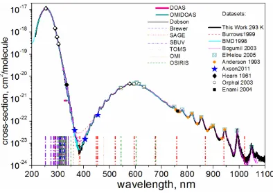
[image:3.595.75.272.260.399.2]Absorption of O2 and O3 attenuates the FUV and UVC in the mesosphere and stratosphere. O2 has a continuous UV absorption band (with decreasing intensity) at the wavelengths of 105 to 252 nm. O3 absorbs continuously (with variable intensity) at the wavelengths of 105 to 1100 nm (See Figure 1) [28, 29]. The release of energy when UV photons are absorbed by O3 is the main source for heating the stratosphere during daytime.
Figure 1. Transmittance Spectrum of O2 in the Visible and Near IR
bands [29]
3.1.2. Absorption of Red and IR Light by O3 and O2 O3 absorbs red light at wavelengths of 540 to 640 nm (see Figure 1) [29]. Absorption of those wavelengths starts in the lower thermosphere. At an altitude of 4.6 km, the cumulative effect of the O3 absorption of red light is considerable (see Figure 2). These absorptions probably intensify the overall feeling of blueness in the sky. Rayleigh scattering is the main reason for blue sky.
Figure 2. The UV–Vis (grey) and Vis–NIR (black) optical depth spectra from sunset observation (3 March 2004, 79:8oN, 80:5oW), shown
for four sample tangent heights. An optical depth of 8 corresponds to a transmission of 0.03% [30]
O3 absorbs IR at wavelengths of 750 to 900 nm and 920 to 1060 nm (the Wulf bands) [29].
O2 absorbs IR at the wavelength s of 1065 nm and 1269 nm [31]. Red light it absorbs at the wavelengths of λ = 627 to 637 nm, λ = 685 to 697 nm and λ = 758 to 772 nm, the A, B and ϒ-bands of O2 respectively [30, 32].
IR absorption by O2 and O3 prevents some of the solar IR and most of the nightglows’ IR from reaching the ground. The release of energy when visible and IR photons and UV photons (from UV nightglows) are absorbed by O3 is an important source of energy for heating the stratosphere during the night.
3.1.3. Attenuation of Solar Light by Inelastic and Elastic Scattering
EUV photons with wavelengths of 10 to 50 nm are screened off by inelastic scattering (in which photons lose energy) already in the thermosphere. Collisions produce photoelectrons [2]. They have enough energy to carry out further ionization reactions [33]. Ionizations caused by EUV creates the ionosphere of Earth.
When photons of UVC, UVB, UVA and blue light collide with N2 and O2 molecules, they are subjected to elastic Rayleigh scattering in the mesosphere, stratosphere and troposphere. At this point photons do not lose energy, only their direction of movement is changed. From the lower stratosphere down the Rayleigh scattering becomes increasingly important.
The deviate portion of solar radiation is called skylight. It comes from all regions of the sky. This means that one can, for example, get a tan even when under a small umbrella at the beach or when skiing on powder snow on a sunny day.
It is estimated that the “sky” portion contributes 15% to 25% of total downwelling irradiance in the blue light region (400 to 500 nm). In the UVA region it contributes 25% to 50%. In the UVB region it contributes 50% to nearly 100% [34].
Only the longer part of UVB (290 ≤ λ ≤ 320 nm), depending on the latitude, reaches the ground [35]. Rayleigh scattering eliminates the most energetic part of the UVB (280 nm ≤ λ ≤ 290 nm), so that only traces of it reach the lower troposphere [36].
3.2. Stratospheric Ozone Layer
3.2.1. Boundaries of the Stratosphere
The height of the tropopause depends on the latitude and the season. During the summer monsoon, the height of the tropopause may be as much as 18 km over southwest Asia. At the midlatitudes, the tropopause is less than 9 to 10 km above sea level. In winter above Antarctica, Siberia and northern Canada its height is 8 km [37]. The lower boundary of the stratosphere varies accordingly.
[image:3.595.75.276.545.699.2]of 47 to 48 km with a standard deviation of 3.2 km [38]. Above Germany its altitude is between 47 and 49 km [39].
3.2 2. Temperature Profile of the Stratosphere
Above Germany the stratospheric temperature increases with altitude at an average of 5 °C per km. The maximum temperature is reached at the altitude range of 45 to 48 km. From the stratopause upwards, the temperature of the mesosphere decreases (see Figure 3).
Figure 3. Nighttime Temperature Profile of the Atmosphere above Germany in June 2005 [39]
The stratopause temperatures above India range from 248 to 279 K with maximum frequency of occurrence in the temperature range of 261 to 262 K [38]. Above Germany the summer stratopause (∼275 K) is slightly warmer than the winter stratopause (∼266 K) [39].
[image:4.595.90.260.196.368.2]During the night the stratosphere cools a bit. Diurnal temperature difference between 20 and 48 km is 1 to 2 degrees. From the stratopause upwards in the mesosphere, the diurnal temperature difference increases (see Figure 4).
Figure 4. Diurnal Temperature Amplitude in the Stratosphere and Mesosphere [40]
3.2.3. Elevations of VMR and Number Density Maxima of Ozone
The maximum volume mixing ratio (VMR) of ozone (9
to 10 ppm) is centered at the altitude of 32 km between 20 oS to 20 oN (see Figure 5). On the other hand, the maximum number density of ozone is centered at altitudes of 15 to 25 km [41]. VMR and number density maxima do not coincide at the same altitude because the density of the air decreases ten times when going from 20 to 35 km [42]. At 20 km, the VMR of 3 ppm contains three times more ozone molecules than the VMR of 10 ppm at 35 km.
During the winter, between the midlatitudes and boreal areas, the number density maximum of ozone (5–6×1012 cm-3) is located at altitudes of 15 to 20 km [43].
Figure 5. Ozone VMR in the Stratosphere and Mesosphere [40]
3.3. Diurnal Variation of the VMR of Ozone in the Stratosphere
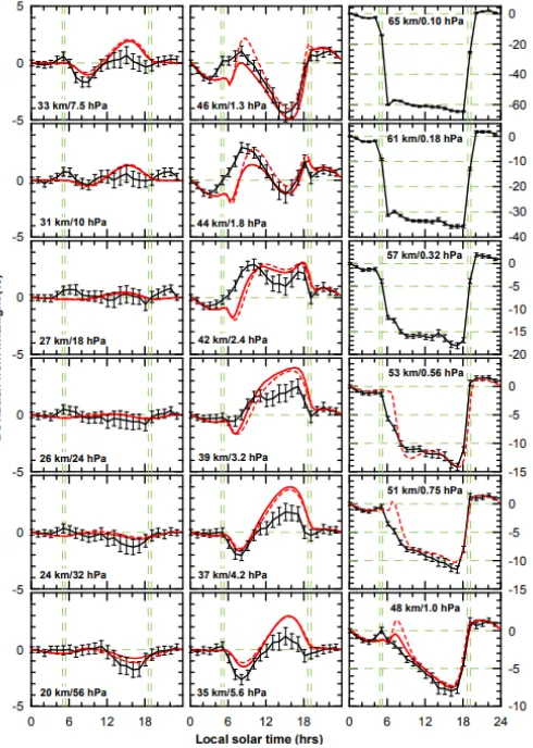
Parrish et al. [44] measured the day–night variation of O3 VMR for each hour of the day over the summer months (June, July, and August) from 1995 to 2013 above Hawaii (see Figure 6).
Between altitudes of 20 to 27 km, the O3 concentrations are more or less the same during the day and night. Within this range UV photons with λ < 252 nm are screened off due to the great absorptive optical density of the atmosphere. So, the dissociation of O2 (1) does not produce O atoms. The photolysis of O3 (2) and the self-decay of ozone are more or less the sole contributors of O atoms. Reaction (3) is able to produce enough new O3, concentration of which remains stable.
A notable exception is the afternoon minimum of O3 at altitudes of 20 to 24 km. The non-absorptive optical density of the atmosphere at this altitude is already so great that the Rayleigh scattering has importance. For this reason, there is more energetic UV radiation available in the afternoon. The photolysis of O3 increases. Reaction (3) is not able to produce enough new O3, concentration of which subsequently decreases.
[image:4.595.325.512.214.396.2] [image:4.595.97.250.519.683.2]photons increases and dissociating of O2 is higher. The produced O atoms fuel the formation of O3 via (3). The O3 concentration reaches its afternoon maximum.
At altitudes of 42 to 46 km, the UV is already in the morning as strong as it is at altitudes of 31 to 39 km at midday. The O3 maximum is now created in the morning. Around midday the production of O atoms increases due to higher O2 dissociation. However, for two reasons this is not enough to boost O3 formation. First, the rate of O3 photolysis increases even more than that of O2 dissociation. Second, the rate of (3) depends on the abundance of a third body M, and therefore on pressure. The air pressure is already so low that the availability of M molecules limits the rate of (3). As a consequence, concentration of O3 is depleted in the afternoon. However, in spite of this the overall ozone turnover is so great that the stratospheric temperature reaches its maximum within the range 45 to 48 km.
From 48 km upwards, UV radiation is intensive enough already from the morning. However, the abundance of M decreases increasingly and so does the rate of (3) as well. Concentration of O3 remains low all day. Overall ozone turnover starts to decrease, and temperature starts to
decrease.
3.4. Excited States of Ozone Molecules
3.4.1. Structure of Ozone Molecule
Ozone is an allotropic form of oxygen constituted of 3 oxygen atoms. It has 24 electrons, of which 6 are in the 3 closed shell inner orbitals, and 18 valence electrons are in 12 outer orbitals [45].
In the ab initio calculations, ozone is considered to have three structural symmetries (a type of conformational isomer): the C2v (open) minimum, the D3h (ring) minimum, and the O (3P) + O2(X
3Σ g
–
[image:5.595.175.420.360.704.2]) dissociation threshold. In the calculations the barrier to isomerization (open → ring → open) is taken to be about 1.3 eV (125.4 kJ/mol) with respect to the dissociation asymptote. The ground electronic state of ozone (in the open minimum conformation) has 1A1 vibrational symmetry [46]. Like O2, O3 molecule has a multitude of electronically excited as well as vibrationally excited states. The excited states have a much weaker O2-O bond and hence may lead to much faster reaction rates with various atoms and molecules.
3.4.2. Electronically Excited Ozone Molecules
The chemistry of the electronically excited ozone molecules is not as straightforward as that of electronically excited oxygen molecules. Already the energy of the lowest excited electronic state of O3 is above its dissociation threshold O (3P) + O2 (X3Σg—). Only the lowest triplet states have so long lifetimes that they likely participate bimolecular reactions in the atmosphere. More highly excited (singlet) states are dissociated immediately. That is why the electronically excited states of O3 are categorized according to the energies of their photolysis products. Relevant reactions in the stratosphere are [45]:
O3 + hν (λ<1180 nm) → O (3P + O2 (X3Σg—) (9) O3 + hν (λ<612 nm) → O (3P) + O2 (1Δg) (10) O3 + hν (λ< 463 nm) → O (
3
P) + O2 (b 1Σ
g +
) (11) O3 + hν (λ< 411 nm) → O (
1
D) + O2 (X 3Σ
g —
) (12) O3 + hν (λ < 310 nm) → O (1D) + O2 (1Δg) (13) Photoexcitation in the Wulf band (9) produces triplet states of O3 that have energies more than 101.4 kJ/mol (1.051 eV). The existence of (rather) distinct absorption spectra actually shows that triplet state ozone molecules do not immediately fall apart. The vertical excitation energy of the triplet states 3B2, 3B1, and 3A2 are 98.4, 156.3 and 170.8 kJ/mol respectively. The radiative lifetimes (RLT) of the 3B2, 3A2 and 3B1 states of ozone are 83.1 s, 0.038 s and 0.200 s, respectively [47].
Photoexcitations in the Chappuis band (10,11) produce singlet states of O3 with energies of more than 195.5 kJ/mol (2.026 eV) and of more than 258 kJ/mol (2.678 eV), respectively. Photoexcitations in the Huggins (12) and Hartley bands (13) produce singlet states of O3 with energies of more than 291.0 kJ/mol (3.016 eV) and 385.9 kJ/mol (3.999 eV), respectively [45].
3.4.3. Vibrationally Excited Ozone Molecules
Ozone has three vibrational quantum numbers: ν1 for the symmetric stretch, ν2 for the bend and ν3 for the antisymmetric stretch. Theoretically, 185 energetically different vibrational states can be calculated up to the dissociation threshold [46].
Ozone absorbs thermal radiation at wavelengths of 9.065, 9.596 and 14.267 µm, at which point the 3 lowest vibrational energy levels of 16O3 are produced: O3(1,0,0) = 1101.9 cm-1 (13.2 kJ/mol), O3(0,1,0) 698.5 cm
-1 (8.4 kJ/mol) and O3(0,0,1) = 1043.9 cm
-1
(12.5 kJ/mol), respectively [46]. The thermal wavelengths that O3 absorbs belong to the outgoing long-wave radiation (OLR) of Earth. It is likely that a considerable proportion of the stratospheric ozone is constantly in vibrationally excited states, except above the poles.
3.4.4. Self-decay of Ozone
In technological applications such as wastewater disinfection technology, the temperature-dependent half-life time (HLT) of ozone is well realized [48]. In the air the HLT of ozone is about 3 months at –50ºC, 18 days at –35 ºC and 8 days at –25 ºC [49].
It has been shown that the decay of ozone follows an empirical mathematical formula. This formula is used to calculate the optimum time intervals when to prepare ozone for a technological application [50].
It has been suggested that collisions with other molecules (bimolecular mechanism) cause the self-decay. The kinetic energy per kelvin (monatomic ideal gas) is KEavg = 3×[R/2] = 3R/2; per mole it is 3.46 kJ/mol at 273K [51]. It can be approximated that at 185 K one mole of ozone is receiving in collisions about 2 kJ of kinetic energy.
Another possibility for self-decay is a unimolecular mechanism via the absorption of thermal radiation. In both cases the acquired energy is a function of temperature. Depending on the temperature, the absorption of thermal radiation may be more important than kinetic collisions in the self-decay of ozone
3.5. Photoexcitation of O2 (X 3Σ
g−
) to Excited Oxygen
Molecules
Vibrationally or electronically excited O2 molecules may undergo reactions that are slow or impossible for ground state O2 molecules. Within its dissociation range, O2 (X3Σg−
)
has up to 26 different vibrational states (ν1–ν26). Energy content of each νi (cumulatively) increases by18.6 to 16.4 kJ/mol. Below its ionization threshold, O2 has several electronically excited states [7]. Each of these states has individual dissociation ranges within which they have individual vibrationally energy levels as well. Table 1 presents the parameters of those electronically excited O2 molecules which have importance in the stratosphere. Additionally, are presented the parameters of O2 (B3Σu−) and O2 (3Πu) molecules, which are photoexcited in the MLT ozone layer as well as above it [52].Table 1. Excitation Energies and Enthalpies of Oxygen Molecules at Different Electronic States [6, 7]
O2 molecule
Excitation energy
kJ/mol Excitation wavelength (nm) Dissociation range kJ/mol X3Σ
g— 0 493.7
a1∆ g
94.3 112.3
1269
1065 399.4
b1Σ+ g
157.0 173.4 189,9
A band: center at 762 nm B band: center at 690 nm
ϒ band: center at 630 nm 336.7 c1Σu— A’1∆u
A3Σ u+
390.8 410.6 418.6
243 < λ < 252 243 < λ < 252 243 < λ < 252
102.9 83.0 74.8 B3Σ
u— 590.6 175–205 93.0
3Π
u 1026.7 107.5–116.5 96.5
In the atmosphere ground state O2 molecules are photoexcited to O2 (a
1Δg
, ν=0 and 1) by IR photons (14) (see Table 1).
O2 (X³Σg−) + hν (λ=1060 nm) →O2 (a1Δg, ν=0) (14) Photoexcitation by red light photons produce O2 (b1Σg+, ν=0, 1 and 2) (15).
O2 (X³Σg−) + hν (λ=760 nm) →O2 (b1Σg+ ν=0) (15) When O2(X3Σg−
)
is photoexcited in the laboratory by UV photons between 243 < λ < 252 nm), vibrationally excited states of O2 (c1Σu−, ν>12, A’1∆u, ν>8, and A3Σu+, ν>7) are produced (16) [56, 57].O2 ( 3Σ−
g) +hν (243<λ <252 nm) → O2 (A 3Σ+
u) (16)
3.6. Stratospheric Daytime Reactions
3.6.1. Photolysis of O3
The photolysis of ozone (2) in the daytime stratosphere is actually comprised of five energetically different pathways (9) to (13). The most important of them is (13). This reaction has been extensively studied. Measurements show that the reaction does not stop (i.e., its quantum yield does not go to 0) even at wavelengths as long as 330 nm if the temperature is cold enough [58]. This is due to the participation of vibrationally excited ozone molecules in the reaction. Owing to this there is a “tail,” the contribution of which enhances the total integrated O (1D) production by more than one third.
3.6.2. The Three-body Recombination
Reaction (3) is the principal ozone-forming reaction at nearly all altitudes in the atmosphere. M represents a non-reactive species, which take up the energy released in (3) to stabilize O3. Without its presence, the produced O3 would immediately return to its respective parts as O and O2.
If O2(X3Σg−, ν = 0) as M molecule receives the released energy, vibrationally excited ground state O2 molecules (up to the level ν = 5) are produced. If the produced O2(X3Σg−, ν = 5) further reacts with O atoms and M is then O2 (b1Σg+),
vibrationally excited ground state O2 molecules up to the level of ν ≥ 18 are produced. According to McGrath and Norrish [59], if (and when) the produced O2(X
3Σ
g−, ν ≥ 18) react with ozone, O (1D) will be produced.
O2(X3Σg−, ν ≥ 18) + O3 → 2O2(X3Σg−, ν =0) + O (1D) (17) This energy pooling pathway may not be a frequent one, but even with a small probability it boosts the dynamics of the stratospheric ozone layer in terms of O (1D) production. 3.6.3. Reactions of Singlet Oxygen Molecules with Ozone When reacting with ozone, singlet oxygen molecules produce O (3P) atom (18, 19).
O2 (1Δg) +O3 (1, 0, 0) → O (3P) + 2O2 (X3Σg−); ∆Ho = −1.0 kJ/mol (18) O2 (b1Σg+) + O3 → O (3P) + 2O2 (X3Σg−);
∆Ho = −47.5 kJ/mol (19) Reaction (19) is expected to be very efficient. An energy transfer process (20) is possible as well. Then excited O3* molecule is formed [11].
O2 (1Δg) + O3 → O2 (X3Σg−) + O3* (20) Singlet oxygen molecules maintain the stability of the stratospheric ozone layer. This is an important expansion of Chapman’s theory of ozone.
3.6.4. Reactions Producing O2 (b1Σg+) in the Stratosphere O2 (b
1Σg+
) is generated in the stratosphere when O2 (A3Σ+u) relaxes (21) [60, 61].
O2 (A3Σ+u) → O2 (b1Σg+) + hν (21) The three-body reaction (22), an energy transfer via O (1D) to O2, is an important source of O2 (b1Σg+) at vibrational levels ν = 0 and 1 in Earth’s atmosphere [62]. O (1D) +O2(X3Σg−) + M → O2 (b1Σg+) + O (3P) + M;
[image:7.595.73.524.91.239.2]preferentially formed with two quanta of vibrational excitation (23) [64]:
O2 (1Δg, ν = 1) + O2 (1Δg ν = 1) → O2 (b1Σg+ ν = 2) + O2 (X3Σg−); ∆H0 = –34.3 kJ/mol (23) At an altitude of 45 to 48 km the dissociation rate of the O2 by UV, the production rates of O(1D), O2(1Δg) and O2(b1Σg+) via the reactions (10) to (13) are the highest [42].
3.7. The Ablation of Meteoroids: An Important Source of Energy for the Nightglows
Important nightglows in the upper atmosphere are the (OI 5577Å) green line nightglow due to the relaxation of O (1S) to O (1D) and the UV nightglows due to the relaxation of O2 (c1Σu−, A’1∆u, and A3Σu+) to ground state O2 molecules. A long-term puzzle in aeronomy has been the energy sources of the nightglows. Energy generated via the ablation of meteoroids may be an important missing link.
3.7.1. The Frequency of Impacts and Elevation of Maximum Ablation
Based on the measurements of cosmic-enriched elements (Ir, Pt, Os and super-paramagnetic Fe) in polar ice cores and deep-sea sediments, the daily accumulation rates of interplanetary dust particles on Earth ranges from 100 to 300 tons [65]. Meteoroids entering at cosmic speed start to ablate due to atmospheric friction. Temperatures may rise even to 3500 ºC for several seconds [66].
The ablation profiles of individual elements differ from each other. The maximum ablation of iron takes place between 95 and 85 km at temperatures of 2000 to 2300 K [67]. During ablations so much energy is generated that the 4.3 µm thermal radiance at an altitude of 92 km is enhanced by about a factor of 50 compared to the 4.3 µm radiation due to the auroral activity [68].
The overall influx of meteoroids to Earth is constant, but on a day-to-day basis the frequency of impacts at a certain latitudinal and longitudinal location changes randomly. 3.7.2. Chemical Reactions Inflicted by Frictional Heat
Generated during Ablation
Any reaction involving molecular oxygen could, in principle, lead to the formation of excited oxygen molecules if sufficient energy were liberated [69]. Heat generated during the ablation of meteoroids is able to produce a wide array of excited oxygen molecules starting from highly excited O2 molecules, such as O2 (3Πu), and ending in the lowest energy states of O2 (b1Σg+) and O2 (a1Δg). According to observations, the UV nightglow due to O2 (A3Σu+) is strongest at 90 to 100 km [70, 71]. It is likely that energy derived from ablations in the MLT layer is producing O2 (c1Σu−, A’1∆u and A3Σu+) which further fuel the UV nightglows.
At temperatures over 2000 K, iron abstracts O atoms from O2 molecules, and excited O (1S) and O (1D) atoms
are then produced. Due to the low overall concentration of iron in meteoroids, the production of O (1S) via this pathway is probably rather small.
The shock-heating over 3500 K excites N2 molecules even to the states of N2 (b’1Σu+) (12.575 eV) and N2 (b1Πu)
(12.849 eV) [72]. It is reasonable to presume that the normal ablation temperature of 2000 to 2300 K would produce excited (metastable) N2 (A3Σ+u), the energy content of which is 9.67 eV. The quenching of N2 (A3Σ+u) by O (3P) atoms produces O (1S) (24) [73].
N2 (A3Σu+) + O (3P) → N2 + O (1S);
∆H0 = –529.3 kJ/mol (24) Measurements during rocket-borne experiments [68] showed that in one leg the emission intensity of the green line nightglow was 10 kilorayleigh (kR), but in another leg it was 30 kR. This kind of variation implies a correlation between O (1S) production and the frequency of meteoroid impacts.
Considering the high proportion of N2 in the air, (24) is an important pathway to produce O (1S) in the night sky at the altitudes of 90 to 100 km to fuel the green nightglow.
3.8. Factors Affecting Stratospheric Night-time Reactions
Astronomical dusk/dawn is divided into civil, nautical and astronomical twilights. At the Equator on the ground, their total duration is 2h20min [74]. Due to the altitude, the
sunset is later (sunrise earlier) by 1 minute for every 1.5 km rise, approximately linearly regardless of latitude [75]. For
this reason, the dusk and dawn at 20 km lasts about 2h33min and at 50 km about 2h53min, a difference of about 3.5%.
During the dusk and dawn, the stratosphere receives visible and IR light from the sun and also from the moon, stars and auroras for production of singlet oxygens and triplet state ozone molecules. Complete darkness or astronomical night is the period between astronomical dusk and dawn [76].At the Equator at 20 km it lasts about 9h27 min, and at 50 km about 9h7min. Then only light from nightglows, moon, auroras and the stars is available. The amount of UV, visible and IR light dramatically decreases. The OLR is an altitude dependent stable source of energy throughout the night.
Moving upwards in the stratosphere the length of the darkness decreases, the intensity of the OLR decreases [68], and the intensity of the light from nightglows, stars and auroras increases. These factors more or less balance the supply of energy, so the stratospheric night-time temperature falls only 1 to 2 degrees between the altitudes of 20 to 48 km.
3.9. Ozone Depletion above the Arctic and Antarctica
Figure 7. The Total Column of Ozone is Shown for the Arctic (NH, top) and the Antarctica (SH, bottom)[77]
3.9.1. Effect of Coldness and the Self-decay of Ozone in Ozone Depletion
The density of ozone is 2.11 g/cm3. Its specific gravity is 1.660 when that of the air is 1.000 [78]. Ozone has no buoyancy anywhere in the atmosphere, so immediately after formation it starts to descend.
It is known that heavy ozone 50O3 (16O18O16O) enriches in the troposphere and lower stratosphere [79]. The descent of ozone is a likely reason for that. Given that in the stratosphere, ozone descends 20 m per day, during the 4 to 6 months of winter it would descend by 2.4 to 3.6 km. In the absence of ozone-producing mechanisms the ozone density then decreases in the lower stratosphere.
The average winter temperature in the Arctic (at 30 hPA or 24.5 km) is –70 ºC [80] and in Antarctica (at 46 hPa or 21km) it is –90 ºC [81]. According to Charles’s law [82],
the volume of a fixed mass of dry gas decreases by 1⁄273
times the volume at 0 °C for every 1 °C fall in temperature. At –90 ºC, the decrease in volume is 33% and at –70ºC it is 25%. The same amount of ozone in moles in a smaller volume means a greater density of ozone. The speed of descent of ozone molecules is greater in Antarctica than it is in the Arctic.
In the Arctic at –70ºC the HLT of ozone would be something like 62 months, the loss of ozone during the winter would be about 6/62×100% = 10%. In the Antarctica, at –90ºC, the HLT of ozone would be about 120 months, and the loss of ozone would be about 6/120×100 = 5%.
Ozone depletion occurs due to the combined effect of the descent of ozone due to gravity (the physical reason) and the self-decay of ozone (the chemical reason). Because ozone depletion is more severe in the Antarctica than it is in the Arctic, the descent of ozone is a more important factor than its self-decay. During the spring when sunshine reaches the polar areas, the ozone layer is recovered.
3.9.2. Lagging of Air Molecules Relative to the Ground on the Rotating Earth
The amount of torque needed to cause any given angular acceleration is proportional to the moment of inertia of a body. It can be thought of as a physical “property” of an object, similar to that of mass [83]. The moment of inertia of Earth’s atmosphere is lower than that of its solid body. Due to this lower angular velocity, the atmosphere does not follow the speed of the solid body while spinning. In other words, the air is lagging. The mass of the atmosphere decreases strongly when moving upwards in the atmosphere. The higher the altitude, the more the air lags. This creates a vertical factor in the lagging of the air relative to the surface.
At the Equator, the rotational speed of Earth is 464 m/s, and at the poles it is 0 m/s. The rotational speed varies according to the cosine of the latitude [84]. At 89 ºN it is 8.1 m/s, and at 80 ºN it is 80.5 m/s. The lower the latitude, the greater the lag of air. This creates a horizontal (latitudinal) factor in the lagging of the air relative to the ground.
Due to the vertical lagging, noctilucent clouds seem to move anticlockwise. However, in fact they are moving clockwise but at a lower speed than the observer on the ground. Due to the combined horizontal and vertical lagging of air, fast moving meteorites seem to create twisted trails. These observations are generally interpreted as winds in the upper atmosphere, even though there are no known and experimentally proven physical factors to generate horizontal winds at those altitudes.
Helium, generated below the ground, moves upwards regardless of the atmospheric pressure or temperature, while ozone descends. These movements (flows or tides) can be interpreted as vertical winds in the upper atmosphere. Due to the lagging of air, this movement creates the illusion of a polar vortex with seemingly faster moving edges and a slower moving center.
3.10. Practical Examples of the Intensity of Ozone Turnover
Above Germany during winter nights, the stratospheric temperature at an altitude of 30 km is even 25 degrees less than during the summer nights (see Figure 8). In the stratopause the difference is only about 10 degrees [39].
[image:9.595.63.283.78.248.2]Figure 8. Seasonal temperature (average June 2002 to July 2007) variation at an altitude of 30 km. Black dots: nightly mean temperatures, blue line: filtered with ±30 day Hanning window, red line: harmonic fit [39]
During the winter months, at altitudes of 74 km and 87 km, the maximum temperature is even 25 degrees higher than in the summer months (see Figure 8). In winter the lower boundary of the MLT ozone layer extends below 87 km and the MMM ozone layer is then formed at altitudes of 70 to 75 km between 45 to 75ºN [86]. (See Figure 9) The ozone turnover in these two ozone layers warms the altitudes of 74 km and 87 km in the winter but not in the summer.
[image:10.595.77.522.382.677.2]4. Conclusions
Ozone absorbs OLR, so most of the atmospheric ozone may constantly be in vibrationally excited states, except above the poles. In addition to the thermal absorption, ozone gains energy via kinetic collisions. Due to these phenomena, ozone is a labile molecule with a distinct temperature-dependent half-life time, and which is ultimately predestined to self-decay.
The existence of ozone in the atmosphere thus needs its constant reformation. The places of most intensive reformation are called ozone layers. There are two global ozone layers, the mesospheric-lower thermosphere (MLT) ozone layer at around 87 to 97 km and the stratospheric ozone layer at around 20 to 50 km. The middle mesospheric ozone maximum (MMM) is formed in the wintertime at an altitude of 70 to 75km. Its location is restricted between the northern mid-latitudes and somewhat north from the Arctic Circle, and symmetrically in the Southern hemisphere.
Excited O2 (a1∆g) and O2 (b1Σg+) are produced in the stratosphere via photoexcitation of red light and IR photons as well as via chemical reactions. At night, the intensity of their production is, of course, much lower. These singlet O2 molecules produce O (3P) when reacting with ozone. They tend to maintain the prevailing ozone concentration and provide stability to the ozone layer.
In the daytime at altitudes of 45 to 48 km, O (1D), O2 (a1∆g) and O2 (b1Σg+) reach their maximum stratospheric concentrations. The ozone turnover as well as the released energy here are both high, which is manifested as the maximum stratospheric temperature between those altitudes.
The density of ozone is 60% more than that of the ambient air. Ozone has no buoyancy in the air and that is why the O3 molecules start to descend immediately when formed. In the 1930s, Chapman calculated that ozone in the stratosphere would descend 20 m per day. At the poles, therefore, ozone descends between 2.4 and 3.6 km during the winter.
Coldness increases the density of O3 relative to the ambient air. Antarctica is clearly colder than the Arctic, so the down drifting of O3 is greater in Antarctica than it is in the Arctic. The descent is the main cause for the depletion of stratospheric ozone above the poles during winter. During the spring when sunshine reaches the polar areas, the ozone layer is recovered.
Acknowledgements
I am very grateful to Matthew Wuethrich from the University of Jyväskylä Language Services for revising the English of the manuscript. I thank my wife Ritva for her support.
REFERENCES
S. Newcomb, A rude attempt to determine the total light of [1]
all the stars, Astrophysical Journal, Vol. 14, 297–312, 1901.
V. Yu. Khomich, A. I. Semenov and N. N. Shefov, Airglow [2]
as an Indicator of Upper Atmospheric Structure and Dynamics, 2008 Springer-Verlag Berlin Heidelberg. ISBN: 978-3-540-75832-7.
M. Kasha, Introductory Remarks: The Renascence of [3]
Research on Singlet Oxygen, In: H. H. Wasserman and R. W. Murray (Eds), Singlet Oxygen, Organic Chemistry A Series of Monographs Vol. 40, Academic Press, New York, 1979. ISBN: 0-12-736650-4.
G. Herzberg, Ein neuartiges “verbotenes” Absorptions [4]
banden system des O2 Moleküls, Naturwissenschaften, Vol.
32, 577, 1932.
H. Kautsky, Quenching of luminescence by oxygen, [5]
Transactions of the Faraday Society, Vol 35, 216–219, 1939.
T. G. Slanger and R. C. Copeland, Energetic Oxygen in the [6]
Upper Atmosphere and the Laboratory, Chemical Reviews,
Vol. 103, No. 12, 4731–4766, 2003. DOI:
10.1021/cr0205311.
P. H. Krupenie, The Spectrum of Molecular Oxygen, Journal [7]
of Physical Chemistry Reference Data, Vol. 1, No. 2, 423– 534, 1972.
S. Chapman, A Theory of Upper Atmospheric Ozone, [8]
Memoirs of the Royal Meteorological Society, Vol 3, 103– 125, 1930.
J. T. N. Jones, Oxygen Chemistry, 211–218, In: B. M. [9]
McCormac (Ed), Atmospheres of Earth and Planets, D. Reidel Publishing Co., Dodrecht, Holland, 1975. ISBN: 90-277-0575-5.
https://www.lenntech.com/library/ozone/decomposition/ozo [10]
ne-decomposition.htm.
P. J. Hay, T. H. Dunning and W. A. Goddard III, Theoretical [11]
evidence for bound electronic excited states of ozone, Chemical Physical Letters, Vol. 23, No. 4, 457–462, 1973.1973.https://doi.org/10.1016/0009-2614(73)89001-3
W. F. J. Evans and E. J. Llewellyn, Measurements of [12]
mesospheric ozone from observations of the 1.27 µ band, Radio Science, Vol. 7, 45–50, 1972.
P. B. Hays and R. G. Roble, Observation of mesospheric [13]
ozone at low latitudes, Planetary and Space Science, Vol. 21, 273–279, 1973.
D. E. Miller and P. Ryder, Measurement of the ozone [14]
concentration from 55 to 95 km at sunset, Planetary and Space Science, Vol. 21, 963–970, 1973.
D. Marsh, A. Smith, G. Brasseur, M. Kaufmann and K. [15]
G. Megie, Ozon. Atmosphäre aus dem Gleichgewicht, p. 47. [16]
Springer-Verlag, Berlin 1989. ISBN: 3-540-5216-9.
M. Allen and M. L. Delitsky, A Test of Odd-oxygen
[17]
Photochemistry Using Spacelab 3 Atmospheric Trace Molecule Observations, Journal of. Geophysical, Research, 96, 12883 –12891, 1991. https://doi.org/10.1029/91JD002 30.
J. Eluszkiewic and M. Allen, A Global Analysis of the [18]
Ozone Deficit in the Upper and Lower Mesosphere, Journal of Geophysical Research, Vol. 98, 1069–1082, 1993.
http://www.mitosyfraudes.org/Ingles/Crista.html. [19]
A. Anduaga, Sydney Chapman on the Layering of the
[20]
Atmosphere: Conceptual Unity and the Modelling of the Ionosphere. Annals of Science, Vol. 66, No. 3, 333–344, 2009. https://doi.org/10.1080/00033790802329455
G. W. van Loon and S. J. Duffy, Environmental Chemistry – [21]
A Global Perspective, Oxford University Press, 49–50, 2005. DOI: 10.1016/0021-9169(72)90061-X
B. J. Finlayson–Pitts and J. R. Pitts Jr. Chemistry of the [22]
Upper and Lower Atmosphere, Academic Press, p. 54 and p. 943, 2000.
R. E. Huffman, Atmospheric Ultraviolet Remote sensing, [23]
Academic Press, NY, 1992. ISBN: 0-12-360390-0.
E. D. Lombardini, M. E. Pacheco-Thompson and M. A. [24]
Melanson, Radiation and Other Physical Agents, Volume II,
Chapter 44, Pages 1421–1503, 2013, In: Haschek and Rousseaux’s Handbook of Toxicological Pathology. ISBN: 978-0-12-415763-7.
P. K. Carroll, R. E. Huffman, J. C. Larrabee and Y. Tanaka, [25]
Absorption by Atomic Nitrogen in the Extreme Ultraviolet, Astrophysical Journal, Vol 146, No. 2, 553–557, 1966.
M. O. Vieitez, T. I. Ivanov, W. Ubachs, B. R. Lewis and C. [26]
A. de Lange, On the complexity of the absorption spectrum of molecular nitrogen, Journal of Molecular Liquids Vol. 141, 110–117, 2008. DOI: 10.1016/j.molliq.2008.01.014.
R. E. Huffman, J. C. Larrabee and Y. Tanaka, New [27]
Absorption Spectra of Atomic and Molecular Oxygen in the Vacuum Ultraviolet. I. Rydberg Series from O I Ground State and New Excited O2 Bands, The Journal of Chemical
Physics, Vol. 46, 2213, 1967. https://doi.org/10.1063/1.184 1026.
S. J. Tu and J. B. Nee, Absorption spectrum of ozone in the [28]
100–200 nm wavelength region, Surface Review and Letters, Vol. 9, 125–128, 2002.
V. Gorshelev, A. Serdyuchenko, M. Weber, W. Chehade, [29]
and J. P. Burrows. High spectral resolution ozone absorption cross-sections – Part 1: Measurements, data analysis and comparison with previous measurements around 293 K, Atmospheric Measuring Techniques, Vol. 7, 609–624, 2014. DOI: 10.5194/amt-7-609-2014.
C.R. Nowlan, C.T. McElroy and J.R. Drummond, [30]
Measurements of the O2 A- and B-bands for determining
temperature and pressure profiles from ACE–MAESTRO: Forward model and retrieval algorithm Journal of Quantitative Spectroscopy & Radiative Transfer Vol. 108 371–388, 2007. DOI: 10.1016/j.jqsrt.2007.06.006.
K. M. Smith and D.A. Newnham, Near-infrared absorption [31]
cross-sections and integrated absorption intensities of molecular oxygen (O2, O2–O2, and O2–N2), Journal of
Geophysical Research, Vol. 105, 7383–7396, 2000.
D. A. Newnham and J. Ballard, Visible absorption [32]
cross-sections and integrated absorption intensities of molecular oxygen (O2 and O4), Journal of Geophysical
Research, Vol. 103, No. D22, 28,801–28,816, 1998.
J. L. Fox, Ion Chemistry, pp. 333–347. In: G. R. North, J.
[33]
Pyle and F. Zhang (Eds), Encyclopedia of Atmospheric Sciences, Vol 1, 2015, Elsevier. ISBN: 978-0-12-382225-3.
Light and the Optical Environment, Princeton University [34]
Press, http://assets.press.princeton.edu/chapters/s2_10281. pdf.webmaster@press.princeton.edu.
http://earthobservatory.nasa.gov/Features/UVB/. [35]
G. Wypych (Ed), Handbook of UV Degradation and [36]
Stabilization, ChemTech Publishing, Toronto, 2015. ISBN: 978-1-895198-86-7.
B. Geerts and E. Linacre, The height of the tropopause, 1997. [37]
http://www-das.uwyo.edu/~geerts/cwx/notes/chap01/tropo. html.
H. Chandra, S. Sharma, Y. B. Acharya and A. Jayaraman, A [38]
Rayleigh lidar study of the atmospheric temperature structure over Mt. Abu, India, The Journal of Indian Geophysical Union, Vol. 9, No. 4, 279–298, 2005.
M. Gerding, J. Hoffner, J. Lautenbach, M. Rauthe, and F.-J. [39]
Lübken, Seasonal variation of nocturnal temperatures between 1 and 105 km altitude at 54oN observed by lidar, Atmospheric Chemistry and Physics, Vol. 8, 7465–7482, 2008. www.atmos-chem-phys.net/8/7465/2008/.
F. T. Huang, R. D. Peters, P. K. Bhartia, H. G. Mayr, S. M. [40]
Frith, J. M. Russell III and M. G. Mlynczak, Temperature diurnal variations (migrating tides) in the stratosphere and lower mesosphere based on measurements from SABER on TIMED, Journal of Geophysical Research, Atmospheres, Vol. 115, No. D16121, 2010. https://doi.org/10.1029/2009J D013698.
NPTL, Module I: Introduction to Meteorology and [41]
Oceanographia, Physics of Atmosphere and Ocean, Atmospheric Science, NPTL National Programme on Technology Enhanced Learning. https://nptel.ac.in/courses /119102007/.
M. Nicolet, Aeronomic Reactions of hydrogen and ozone, pp. [42]
1–51. In: G. Fiocco (Ed), Mesospheric Models and Related Experiments, D. Reidel, Dodrecht, Holland, 1971. ISBN: 90-154737.
E. Kyrölä, J. Tamminen, G. W. Leppelmeier, V. Sofieva, S. [43]
Hassinen, A. Seppala, P. T. Verronen, J. L. Bertaux, A. Hauchecorne, F. Dalaudier, D. Fussen, F. Vanhellemont, O. Fanton d’Andon, G. Barrot, A. Mangin, B. Theodore, M. Guirlet, R. Koopman, L. Saavedra de Miguel, P. Snoeij, T. Fehr, Y. Meijer, and R. Fraisse, Nighttime ozone profiles in the stratosphere and mesosphere by the Global Ozone Monitoring by Occultation of Stars on Envisat, Journal of Geophysical Research, Vol. 111, D24306, 2006. DOI: 10.1029/2006JD007193.
Frith, N. A. Kramarova, B. J. Connor, G. E. Bodeker, L. Froidevaux, M. Shiotani, and T. Sakazaki, Diurnal variations of stratospheric ozone measured by ground-based microwave remote sensing at the Mauna Loa NDACC site:
measurement validation and GEOSCCM model
comparison, Atmospheric Chemistry and Physics, Vol. 14, 7255–7272, 2014. https://doi.org/10.5194/acp-14-7255-20 14.
S. Yu. Grebenshcikov, Z.-W. Qu, H. Zhue and R. Schinke, [45]
New theoretical investigations of the photodissociation of ozone in the Hartley, Huggins, Chappuis and Wulf bands, Physical Chemistry Chemical Physics, Vol. 9, 2044–2064, 2007.
R. Siebert, P. Fleurat-Lessard, R. Schinke, M. Bittererova [46]
and S. C. Farantos, The vibrational energies of ozone up to the dissociation threshold: Dynamics calculations on an accurate potential energy surface, The Journal of Chemical Physics Vol. 116, No. 22, 9749–9767, 2002. https://doi.org/10.1063/1.1473664.
H. Ågren, O. Vahtras and B. Minaev, Response Theory of [47]
Calculations of Spi-Orbit Coupling Phenomena in Molecules. In: P.-O. Löwdin, J. S. Sabin and M. C. Zerner (Eds), Advances in Quantum Chemistry, Vol. 27, p. 106, 1996. Academic Press. ISBN: 0-12-034827-6.
D. McClurkin and D.E. Maier, Half-life time of ozone as a [48]
function of air conditions and movement, 10th International Working Conference on Stored Product Protection, Julius-Kühn-Archiv, 381–385, 425, 2010. DOI: 10.5073/jka.2010.425.167.326.
Ozone Data & Conversion Tables, Plasma & Reactive Gas [49]
Solutions. https://www.mksinst.com/docs/UR/astexozoned ata.pdf
V. Gorshlev, Absorption spectroscopy of atmospheric [50]
species (ozone) https://www.msc-ep.uni-bremen.de/service s/lectures/practicals/pr_ozone_2016.pdf.
https://en.wikipedia.org/wiki/Kinetic_theory_of_gases. [51]
K. Hänninen, The Role of Excited Oxygen Molecules in the [52]
Formation of the Secondary Ozone Layer at 87 to 97 km, Environment and Ecology Research Vol. 1, 74–85, 2018. http://www.hrpub.org DOI: 10.13189/eer.2018.060107.
R. P. Wayne, Reactions Involving Excited States of O and [53]
O2, pp. 125–132. In: B. M. McCormak (Ed), Physics and
Chemistry of Upper Atmosphere, D. Reidel, Dodrecht, Holland, 1973. ISBN: 978-94-010-2542-3.
M. E. Jimenez-Hernandez, F. Manjon, D. Garcia-Fresnadillo [54]
and G. Orellana, Solar Water disinfection by singlet oxygen molecule by singlet oxygen photogenerated with Ru(II) sensitizers, Solar Energy, Vol. 80, No 10, 1382–1387, 2006.
A. M. Starik, Innovations in combustion technologies for [55]
propulsion 26th International Congress of the Aeronautical Sciences, 2008 Central Institute of Aviation Motors,
Moscow, Russia.
https://www.icas.org/media/pdf/ICAS%20Congress%20G eneral%20Lectures/2008/ICAS%202008%20Starik.pdf.
R. A. Copeland, K. Knutsen and T. G. Slanger. Using [56]
Laser-Induced Fluorescence to Study molecules of Atmospheric importance pp. 318–325. In: The Proceedings of the International Conference on Lasers ´93- Lake Tahoe,
NV, 1993.
R. A. Copeland, K. Knutsen, M. E. Onishi and T. Yalcin, [57]
Collisional removal of O2(c1Σu−, ν=9) by O2, N2 and He,
The Journal of Chemical Physics, Vol 105, No 23, 10349– 10355, 1996.
Y. Matsumi, F. J. Comes, G. Hancock, A. Hofzumahaus, A. [58]
J. Hynes, M. Kawasaki, and A. R. Ravishankara, Quantum yields for production of O (1D) in the ultraviolet photolysis of ozone: Recommendation based on evaluation of laboratory data, Journal of Geophysical Research, Vol. 107,
No. D3, ACH 1-1–ACH 1-12, 2002.
https://doi.org/10.1029/2001JD000510.
W. D. McGrath and R. G. W. Norrish, Production of [59]
Vibrationally Excited Oxygen Molecules in the Flash Photolysis of Ozone, Nature, Vol. 180, 1272–1273, 1957. DOI: 10.1038/1801272b0.
G. Bednarek, R. P. Wayne, J. Wildt, and E. H. Fink, [60]
Erratum,The yield of O2(b1Σg+, ν = 0) produced by
quenching of O2(A3Σg+, ν = 8) by O2, [Chem. Phys., Vol.
185, 251–261, 1994], Chemical Physics, Vol. 222, 113–114, 1997.
K. S. Kalogerakis, A. Totth, P. C. Cosby, T. G. Slanger and [61]
R. A. Copeland, Laboratory studies of the production of highly vibrationally excited O2(a1∆g and b1Σg+) from
O2(A3Σu+) relaxation, EOS Transactions of the American
Geophysical Union, Vol. 81, F944, 2000.
A. Dušan, R. A. Pejaković, T. Copeland, G. Slanger and K. [62]
S. Kalogerakis: O2 (b 1Σ
g +
, ν = 0, 1) relative yields in O(1D) O2 energy transfer. The Journal of Chemical Physics,
Vol. 141, 024303, 2014. DOI: http://dx.doi.org/10.1063/1.4885721.
R. P. Wayne, The photochemical formation of electronically [63]
excited oxygen molecules in the atmosphere, Quarterly Journal of Royal Meteorological Society, Vol. 93, No. 395, 69–78, 1967. https://doi.org/10.1002/qj.49709339506.
U. Schurath, The energy pooling reaction 2O2 (1Δg) → O2
[64]
(3Σ−g) + O2 (1Σ+g) formation, relaxation, and quenching of
vibrationally excited O2(1Σ+g), Journal of Photochemistry,
Vol 4. No. 3, 215–226, 1975. https://doi.org/10.1016/0047-2670 (75)80007-4.
J. M. C. Plane, Cosmic dust in the Earth's atmosphere, Chemical [65]
Society Reviews., Vol. 41, 6507–6518, 2012. DOI: 10.1039/C2CS35132C.
V. Della Corte, F. J. M. Rietmeijer, A. Rotundi, M. Ferrari [66]
and P. Palumbo, Meteoric CaO and carbon smoke particles collected in the upper stratosphere from an unanticipated source, Tellus B: Chemical and Physical Meteorology, Vol. 65, No. 1, Article: 20174, 2013. DOI: 10.3402/tellusb.v65i 0.20174, https://doi.org/10.3402/tellusb.v65i0.20174.
T. Vondrak, J. M. C. Plane, S. Broadley and D. Janches, A [67]
chemical model of meteoric ablation, Atmospheric Chemistry and Physics, Vol. 8, 7015–7031, 2008. www.atmos-chem-phys.net/8/7015/2008/.
A. T. Stair, Jr, J. C. Ulwick, K. D. Baker and D. J. Baker, [68]
R. P. Wayne, Singlet oxygen molecule, pp. 311–371. In: J. N. [69]
Pitts, G. S. Hammond and W. A. Noyes (Eds), Advances in Photochemistry, New York, 1969.
I. C. McDade and J. E. Llewellyn, The Altitude Dependence [70]
of the O2 (A3Σu+) Vibrational Distribution in the Terrestrial
Nightglow, Planetary and Space Science, Vol. 30, No 11, 1135–1136, 1982.
D. P. Murtaugh, I. C. McDade, R. G. H. Greer, J. Stegman, G. [71]
Witt and E. J. Llewellyn, Eton 4: An Experimental Investigation of the Altitude Dependence of the O2(A3Σu+)
vibrational Populations in the Nightglow, Planetary and Space Science, Vol. 34, No. 9, 811–817, 1986.
A. Lofthus and P. Krupenie, The Spectrum of Molecular [72]
Nitrogen, Journal of Chemical Reference Data, Vol. 6, No. 1, 113–2307, 1977.
J. A. Meyer, D. W. Setser and D. H. Stedman, Excitation of [73]
the auroral green line of atomic oxygen 1S→1D by N2(A3Σ+u), Astrophysical Journal, Vol. 157, 1023–1025,
1969
https://www.timeanddate.com/astronomy/astronomical-twil [74]
ight.html.
http://curious.astro.cornell.edu/about-us/161-our-solar-syste [75]
m/the-earth/day-night-cycle/189-how-do-sunrise-and-suns et-times-change-with-altitude-intermediate.
https://en.wikipedia.org/wiki/Night.
[76]
http://www.memagazine.org/backissues/membersonly/octo [77]
ber98/features/stratos/stratos.html.
Mine Gases: Specific Gravity. https://miningquiz.com/dow [78]
nload/GasSpecificGravity.htm
J. M. Flaud and R. Bacis, The ozone molecule: Infrared and [79]
microwave spectroscopy, Spectrochimica Acta Part A, Vol. 54, 3–16, 1998.
K. Labitzke and B. Naujokat, The Lower Arctic
[80]
Stratosphere in Winter since 1952, SPARC Newsletter, 15, 11-14, 2000.https://www.sparc-climate .org/fileadmin/customer/6_Publications/Newsletter_PDF/1 5_SPARCnewsletter_Jul2000_redFile.pdf.
G. Günther, D. S. McKenna and R. Spang, Meteorological [81]
conditions of the stratosphere for the CRISTA 2 campaign, August 1997, Journal of Geophysical Research, Vol. 107,
No. D23, CRI 12-1–CRI 12-10, 2002. DOI:
10.1029/2001JD000692.
https://en.wikipedia.org/wiki/Charles%27s_law. [82]
https://en.wikipedia.org/wiki/Moment_of_inertia. [83]
https://image.gsfc.nasa.gov/poetry/ask/a10840.html. [84]
E. Kyrölä, GOMOS/Envisat overview, Day 2 Lecture 5 [85]
Basics/Instruments, Dragon advanced training course in atmosphere remote sensing, ESA, NASCC, 2003. https://earth.esa.int/dragon/D2_L5_Kyrola.pdf.
L. Moreira, K. Hocke, and N. Kämpfer, Comparison of [86]
![Figure 3. Nighttime Temperature Profile of the Atmosphere above Germany in June 2005 [39]](https://thumb-us.123doks.com/thumbv2/123dok_us/8788982.908376/4.595.97.250.519.683/figure-nighttime-temperature-profile-atmosphere-germany-june.webp)
![Table 1. Excitation Energies and Enthalpies of Oxygen Molecules at Different Electronic States [6, 7]](https://thumb-us.123doks.com/thumbv2/123dok_us/8788982.908376/7.595.73.524.91.239/excitation-energies-enthalpies-oxygen-molecules-different-electronic-states.webp)
![Figure 7. The Total Column of Ozone is Shown for the Arctic (NH, top) and the Antarctica (SH, bottom) [77]](https://thumb-us.123doks.com/thumbv2/123dok_us/8788982.908376/9.595.63.283.78.248/figure-total-column-ozone-shown-arctic-nh-antarctica.webp)

