A Rising Market and Capital Structure Decisions

(1)

A Rising Market and Capital Structure Decisions

*

Hui Yang1, Mohammad Meysami2, Alex Meisami3,*

1

Financial Analyst at Indratech LLC, Elkhart, Indiana, USA 2

Ph.D. Candidate, Department of Mathematical and Statistical Sciences, University of Colorado Denver, USA 3

Associate Professor of Finance, Leighton School of Business and Economics, Indiana University South Bend, USA

Abstract

This paper examines capital structure decisions in the 1990s. We test a number of capital structure theories and find notable differences between investment- and junk-grade issuers in this period. Consistent with the trade-off theory, 67% of junk-grade issues were equity as opposed to only 9% of investment-grade issues. In addition, consistent with the trade-off theory, for junk-grade issuers, we find a direct relationship between collateral and debt issuance and an inverse relationship between debt issuance and the treasury yield. However, contrary to the predictions of the trade-off theory, we do not find similar evidence for investment-grade issuers. Moreover, our analysis suggests that junk-grade issuers are concerned with the wealth-transfer consequences of choosing equity over debt; this does not seem to be the case for investment-grade issuers. We find some evidence in support of market timing and little evidence for the pecking order theory or the equity undervaluation hypothesis.

Keywords

Capital Structure, Junk-grade,

Investment-grade

1. Introduction and Prior Literature

Review

According to the trade-off theory, a company’s capital structure is formed by the trade- off between tax savings of debt and deadweight costs of bankruptcy. This leads to an optimal leverage for which a firm’s value is maximized. Another word, a company’s worth is a concave function of its leverage.

A competing theory, pecking order, was proposed by Myers et al. [1, 2]. Pecking order argues that companies follow a pecking order when choosing between debt and equity for external funding. Firms issue equity only after they have exhausted their internal funds, short- and long-term debt capacity. Consequently, issuing equity is the costliest form of financing because of the highest level

of asymmetric information associated with equity issuance. Market timing hypothesis asserts that firms opportunistically issue equity after a period of increase in their stock price. It predicts negative returns after stock issues. Equity undervaluation hypothesis suggests that firms issue debt when their equity is undervalued. It predicts positive equity returns after debt issues. Finally, according to the wealth transfer hypothesis of capital structure, issuing equity transfers wealth from existing shareholders to creditors. Another word, after stock issuance, the new equity cushion reduces the default risk that causes higher bond values and effectively transferring wealth from stock to bondholders. Eberhart and Siddique relate the negative reaction following stock issues to the wealth transfer concerns (from existing shareholders to creditors) [3].

This paper contributes to the literature by focusing on a specific period of steady rise in the stock market. We test a number of capital structure theories in order to understand the underlying reasons as to why companies preferred debt over equity or vice versa during a decade of strong investor sentiment: the 1990’s bull market. In doing so, we compare investment- and junk-grade firms and find distinguishing differences between the two groups. The paper is organized as follows: section 2 describes the data and sample construction. We discuss the results in section 3 and conclude in section 4.

2. Data, Sample, and Methodology

(2)

company’s rating, the observation was dropped. This is the case for both debt and equity issues. When a subsequent debt or equity issuance occurs within 20 days of the first issuance, the issue is dropped.

Further, for each issue, we require the price data (from CRSP) to be available 250 days (excluding weekends) before and after issue else, we drop the issue. Similarly, we require all of our control variables, i.e. collateral, profitability, market-to-book, and leverage to be available for all the issuing companies or the issue is dropped. Table 1 presents the sample, a total of 1891 debt issues and 519 equity issues in the 1990-1999 period. Later, we drop all the debt issues used to refinance the debt in place because debt refinancing does not effectively change the capital structure. This reduces the debt sample to 1346 observations.

Table 1. Distribution of Offerings by Year

Debt Equity

All No Debt Refinancing All

1990 101 73 30

1991 202 131 76

1992 206 129 73

1993 233 151 90

1994 119 81 53

1995 186 129 55

1996 189 144 56

1997 217 184 44

1998 260 201 13

1999 178 123 29

Total 1891 1346 519

Marginal tax rates are downloaded from John Graham’s website. As a substitute for leverage, we calculate and use leverage-deficit as a control variable in our analysis. This follows Hovakimian et al. [4] and Leary et al. [5]. They show that the deviation from leverage ratio is a better determinant of capital structure choices than leverage. Lastly, we calculate post-issue firm-specific return as the difference between the firms and market holding-period returns (HPRs) over a one-year period after issue.

2.1. General Sample Characteristics

Our initial sample consists of 519 equity issues and 1891 debt issues in the 1990-1999 period (Table 1). Out of 1891 debt issues, 545 were used to refinance existing debt and therefore were dropped. Our final sample consists of 1346 debt issues and 519 equity issues that we use in our analysis.

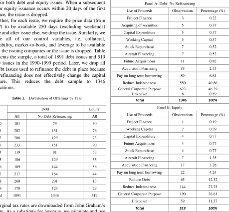
Table 2 shows how the overall proceeds from debt (no refinancing) and equity issues were used during the 1990-1999 period.

Table 2. Primary Use of Proceeds Obtained from SDC

Panel A: Debt- No Refinancing

Use of Proceeds Observations Percentage (%)

Project Finance 3 0.22

Acquiring of securities 5 0.37

Capital Expenditure 5 0.37

Working Capital 5 0.37

Stock Repurchase 7 0.52

Aircraft Financing 7 0.52

Future Acquisitions 11 0.82

Acquisition Financing 33 2.45

Pay on long term borrowing 89 6.61

Reduce Indebtedness 550 40.86

General Corporate Purpose Unknown

623 8

46.29 0.59

Total 1346 100%

Panel B: Equity

Use of Proceeds Observations Percentage (%)

Project Finance 1 0.19

Working Capital 2 0.39

Capital Expenditure 4 0.77

Future Acquisitions 4 0.77

Stock Repurchase 4 0.77

Aircraft Financing 7 1.35

Acquisition Financing 17 3.28

Pay on long term borrowing 22 4.24

Reduce Debt 65 12.52

Reduce Indebtedness 144 27.75

General Corporate Purpose 190 36.61

Unknown 59 11.37

Total 519 100%

[image:2.595.80.540.93.518.2]

(3)

specifics of the General Corporate Purpose and the number of unknown issues for the equity sample.

On the surface, just a sheer volume of debt issues, 1346 and equity issues 519 in this period (2.6 debt issues for every equity issue) could indicate a pecking order; firms issue equity as the last resort due to asymmetric information and the agency costs associated with equity issues. Equity undervaluation hypothesis can also justify debt preference if we observe positive stock abnormal returns after debt issues. We will test this hypothesis.

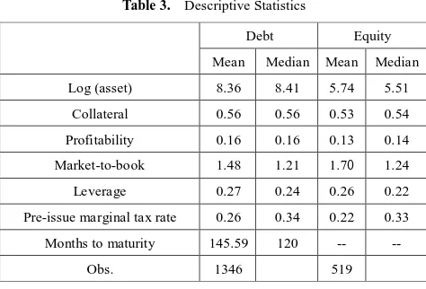
Table 3. Descriptive Statistics

Debt Equity

Mean Median Mean Median

Log (asset) 8.36 8.41 5.74 5.51

Collateral 0.56 0.56 0.53 0.54

Profitability 0.16 0.16 0.13 0.14

Market-to-book 1.48 1.21 1.70 1.24 Leverage 0.27 0.24 0.26 0.22

Pre-issue marginal tax rate 0.26 0.34 0.22 0.33

Months to maturity 145.59 120 -- --

Obs. 1346 519

Table 3 compares the general characteristics of our control variables. Variables in this table are defined in the Appendix. Graham marginal tax rates are recorded as of one year before the issue date [6]. Debt maturity is calculated by extracting issue date and maturity date from SDC. The table shows that debt issuers are more sizable than equity issuers. Size is measured by the log of assets. The mean (median) size for the debt issuers is 8.36 (8.41) as opposed to 5.74 (5.51) for equity issuers. Debt issuers show slightly higher mean (median) profitability than equity issuers; 0.16 (0.16) versus 0.13 (0.14), and they are slightly more leveraged than equity issuers are. Debt issuers have mean (median) leverage of 0.27 (0.24) relative to equity issuers, 0.26 (0.22).

Consistent with the trade-off theory, debt issuers have lower mean market-to-book ratio than equity issuers, 1.48 versus 1.70. However, median market-to-book ratios are more comparable between the two groups, 1.21 for debt issuers versus 1.24 for equity issuers. In addition, consistent with the trade-off theory, debt issuers have pre-issue mean marginal tax rate of 0.26 versus 0.22 for equity issuers. However, the medians are more comparable, 0.34 versus 0.33. The mean (median) maturity for the debt issues is 12 (10) years.

3. Results

Panel A in Table 4 provides a logit comparison of debt-equity choices for our final sample of 1865 observations comprised of all equity issues (519) and debt issues with no refinancing (1346). The dependent variable is either 1 if debt was issued or 0 if equity was issued. The independent variables are defined in the Appendix. The dependent variable is 1 for debt issues and 0 for equity issues. Leverage deficit, Market-to-book, Collateral, Profitability, and Prior 1 yr. firm-specific return are winsorized at the 1% level. Appendix contains a complete description of these variables. *, **, and *** indicates significance at 10%, 5% and 1% level.

Consistent with the trade-off theory the leverage deficit (median industry leverage minus firm’s leverage) has a positive and significant coefficient. Assuming that the industry leverage is a reasonable substitution for a firm’s optimal leverage, this shows that underleveraged firms attempt to issue additional debt to get closer to their optimal leverage ratio. This is in line with the predictions of the trade-off theory. In addition, Table 4 shows that bigger (measured by log (assets)) and more profitable firms are expected to issue more debt. This is also consistent with the trade-off because bigger and more profitable firms tend to have higher marginal tax rates and thus more incentive to issue debt instead of equity. However, for the overall sample, higher rates (T-bill) do not seem to deter firms from issuing less debt. The coefficient for T-bill is negative (in line with trade-off) but insignificant. The coefficient for collateral is positive (in line with trade-off) but insignificant.

Consistent with market timing, firms with higher momentum (pre-runup) issue more equity and consistent with the trade-off theory, firms with higher growth options (measured by market-to-book ratio) tend to issue more equity. The coefficient is significant at the 5% level. Further, bullish markets seem to encourage firms to issue more equity; the coefficients for pre-mkt and pre-runup are significant at 1% level.

[image:3.595.55.292.210.371.2]

(4)

Table 4. Logit Comparison of Debt and Equity Issues

Panel A: All (n=1865)

Variable Estimate Standard Error Wald Chi-Square Pr > Chi-Square sig

Intercept -3.068 0.7472 16.8597 <.0001 ***

Def_Mlev 1.6081 0.4309 13.9267 0.0002 ***

MB -0.192 0.0978 3.8542 0.0496 **

Collateral 0.4451 0.3542 1.5797 0.2088

Profit 3.5972 1.143 9.9041 0.0016 ***

Log-asset 0.829 0.0466 316.1626 <.0001 ***

TBILL -0.0949 0.0767 1.5312 0.2159

spread -1.618 0.4314 14.0666 0.0002 ***

pre_Mkt -1.6332 0.4387 13.8577 0.0002 ***

pre_runup -1.1837 0.1544 58.7644 <.0001 ***

Panel B: Investment grade (n=1254)

Intercept -1.7498 1.2168 2.0678 0.1504

Def_Mlev 2.1835 0.7806 7.8251 0.0052 ***

MB -0.4494 0.1708 6.9263 0.0085 ***

Collateral -1.2393 0.5567 4.955 0.026 **

Profit 9.2302 2.4103 14.6649 0.0001 ***

Log-asset 0.6301 0.0901 48.9465 <.0001 ***

TBILL 0.1517 0.1205 1.5847 0.2081

spread -1.756 0.6205 8.0093 0.0047 ***

pre_Mkt -1.9115 0.6175 9.5826 0.002 ***

pre_runup -1.4153 0.3028 21.8546 <.0001 ***

Panel C: Junk grade (n=611)

Intercept -0.8984 1.1572 0.6027 0.4375

Def_Mlev 0.3788 0.5804 0.4261 0.5139

MB -0.0901 0.1314 0.4706 0.4927

Collateral 1.704 0.4921 11.9907 0.0005 ***

Profit -0.6984 1.2866 0.2947 0.5872

Log-asset 0.5301 0.0783 45.834 <.0001 ***

TBILL -0.2963 0.1125 6.94 0.0084 ***

spread -2.4981 0.8402 8.8398 0.0029 ***

pre_Mkt -0.6267 0.6939 0.8157 0.3664

pre_runup -0.94 0.1807 27.055 <.0001 ***

Results in Panel B for the subsample of 1254 investment grade firms are very similar to Panel A. With the exception of collateral, all other coefficients have the same sign and similar statistical significance. Surprisingly, collateral has a negative sign and is significant at 5% level suggesting that investment-grade firms with more collateral issue more equity. This cannot be explained by the capital structure theories tested in this paper.

We observe several differences in panel C when we run the logit regression for the junk-grade firms. First,

[image:4.595.62.540.92.616.2]

(5)

junk-grade firms. This is also inconsistent with the predictions of the trade-off theory. Interestingly, unlike the investment-grade firms, junk-rated firms are more sensitive to the yield curve (T-bill). Panel C suggests that during the 1990-1999 period as rates increased junk-rated firms made fewer debt issues. The coefficient for the T-bill is significant a 1% level. This is consistent with the trade-off; as rates go up the dead-weight costs of bankruptcy exceed the tax saving benefits of debt. Junk-grade firms behave similarly to the investment-grade firms when it comes to pre-runup and credit spread. Overall, we find mixed results for the trade-off theory.

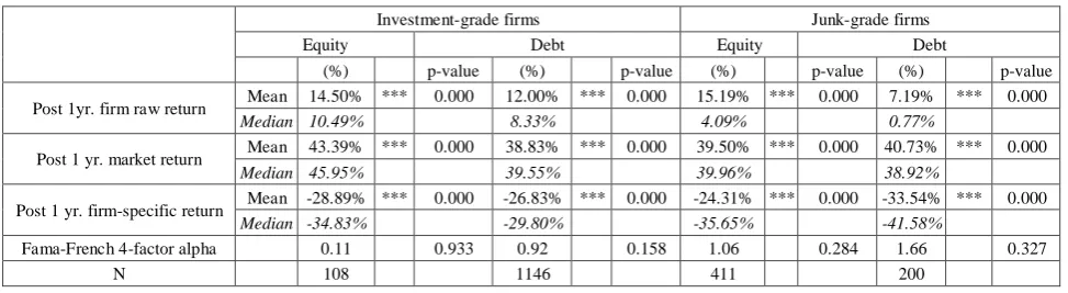
Table 5 presents firm and market returns post issue. First, 67% of junk-grade firms issued equity (411/611) as opposed to 9% of investment-grade firms (108/1254). This is consistent with the trade-off because junk-grade firms have lower marginal tax rate and higher cost of bankruptcy. Further, junk and investment-grade issuers’ mean and median raw and firm-specific returns (firm’s raw return minus market return) are presented and compared. As expected, consistent with the bull market wave of the 1990s, post-issue market returns are positive for all the categories (1% significance level).

Investment-grade as well as junk- grade equity issuers face post-issue firms-specific returns that are negative at 1% significance level. Several theories in capital structure can explain this finding. According to the market-timing hypothesis, overvalued equity incentivizes companies to take advantage of the good market conditions by issuing equity. The negative post-issue returns are consistent with the market-timing hypothesis as it predicts that a firm’s stock price to revert to its intrinsic value following the issuance of overvalued equity. The pecking order theory also predicts this. As the least desirable way of external financing, due to its agency costs, equity is always more expensive than debt. However, this argument is weakened when we look at junk-grade issuers with logically higher agency costs than investment-grade issuers. Table 5 shows that firm-specific returns for junk-grade debt issues are negative and even 9.23% lower than junk-grade equity issues.

As was the case for equity issuers, both investment and junk-grade debt issuers have negative and significant

post-issue returns. Among the four categories, junk-grade debt issuers’ stock price drops the most post-issue. While negative stock returns after debt issues are well documented in the literature, Spiess and Affleck-Graves find that straight, as well as convertible debt issuers, also face negative post-issue stock returns [7]. They also find that this problem is more severe for younger, smaller, and junk-grade issuers and NASDAQ-listed firms have the same problem. They conclude that similar to equity issues, debt offerings also signal overvaluation.

Next, in both categories, equity issuers’ raw returns outperform those of debt issuers. We also observe that for investment-grade firms, consistent with the equity undervaluation hypothesis, debt issuers show higher firm-specific post-issue returns than equity issuers. Yet interestingly, for the junk sample we observe the opposite. That is, junk-grade post-issue firm-specific returns are higher for equity issuers than debt issuers. This observation cannot be explained by the equity undervaluation hypothesis since according to this hypothesis, debt issues are caused by equity undervaluation. Therefore, Table 5 provides evidence against the equity undervaluation hypothesis for the junk-grade issues.

Finally, we use Carhart 4-factor model [8] that is similar to Fama-French 3-factor model [9] with an added factor (momentum). We do not find any statistical significance for post-issue returns using this model.

In Table 6, we present three-day cumulative abnormal returns (CAR3) around the announcement of the security issues for the investment- and junk- grade samples. Mean and median CAR3 is negative and significant at 1% for all the categories with the exception of junk-rated debt issues. In addition, junk-rated equity issues show the highest reaction (-1.59% CAR3) followed by investment-grade equity issues (-1.17% CAR3).A more negative market response to equity issues is consistent with pecking order because equity is the least desirable source of external financing according to the pecking order. However, post-issue firm-specific retunes presented in Table 5 do not support the notion that in the long run debt financing, especially junk-debt, has any advantage over equity financing.

Table 5. Post-issue Stock Returns

Investment-grade firms Junk-grade firms

Equity Debt Equity Debt

(%) p-value (%) p-value (%) p-value (%) p-value

Post 1yr. firm raw return Mean 14.50% *** 0.000 12.00% *** 0.000 15.19% *** 0.000 7.19% *** 0.000

Median 10.49% 8.33% 4.09% 0.77%

Post 1 yr. market return Mean 43.39% *** 0.000 38.83% *** 0.000 39.50% *** 0.000 40.73% *** 0.000

Median 45.95% 39.55% 39.96% 38.92%

Post 1 yr. firm-specific return Mean -28.89% *** 0.000 -26.83% *** 0.000 -24.31% *** 0.000 -33.54% *** 0.000

Median -34.83% -29.80% -35.65% -41.58%

Fama-French 4-factor alpha 0.11 0.933 0.92 0.158 1.06 0.284 1.66 0.327

[image:5.595.55.542.615.748.2]

(6)

In Table 4 we got mixed results when we tried to explain the debt-equity choices of junk-grade firms by the trade-off theory. In Table 6, junk-grade debt issuers are the only group with no negative stock reaction to the announcement of the issue. In fact, the mean CAR3 is positive (0.14%) although not significant. This observation is consistent with the wealth-transfer notion as elaborated by Eberhart and Siddique [3]. The authors show that adverse stock response to equity issue announcements signals wealth transfer concerns. According to the wealth transfer hypothesis, shareholders of risky firms (such as junk-grade firms) are more inclined to issue debt because issuing equity will result in a wealth-transfer from existing stockholders to bondholders by reducing the default risk. The results in Table 6 are consistent with their finding. The stock reaction to the announcement of junk-grade equity issues is -1.59% and significant at 1% as opposed to a positive and insignificant reaction observed for junk-grade debt issues.

Table 6. Analysis of Stock Reaction to Announcement of Security Issues

N CAR3 z-statistics

Investment equity 108 Mean -1.17% *** -4.33 Median -1.52%

Investment debt 1146 Mean -0.25% *** -3.02 Median -0.34%

Junk equity 411 Mean -1.59% *** -4.91 Median -1.67%

Junk debt 200 Mean 0.14% 0.95 Median -0.32%

4. Conclusions

In this paper, we attempt to understand the underlying reasons for debt versus equity issues during the 1990s. We find that debt issuers used approximately 87% of proceeds for general corporate purposes or to repay debt. Almost

77% of equity issuers used the proceeds for the same purpose. On the surface, higher debt issues in this period are in line with the predictions of the pecking order theory; but our subsequent analysis does not support pecking order. In addition, debt issuers were larger, slightly more profitable, and more leveraged than equity issuers. Consistent with the trade-off theory, debt issuers had higher marginal tax rates and lower growth options measured by market-to-book ratio. Additionally, consistent with the trade-off, we find a negative relationship between debt issuance and uncertainty regarding economic prospects as measured by the higher credit spread.

We show that 67% of junk-grade firms issued equity as opposed to 9% of investment-grade firms. While this is in line with the trade-off theory because junk-grade firms have lower marginal tax rates and higher costs of bankruptcy, we find evidence that junk-grade firms avoid issuing equity also due to wealth-transfer concerns. According to the wealth-transfer hypothesis, an equity issuance will benefit bondholders at the expense of equity holders by lowering the default risk. In contrast, we show that such wealth transfer concerns do not seem to alarm investment-grade issuers. We also find evidence in support of the market timing hypothesis since firms with higher stock price momentum were more likely to issue equity. We find little evidence in support of pecking and equity undervaluation.

We are not able to explain the following: first, investment-grade firms with higher collateral issued more equity (but consistent with the trade-off theory, junk-grade firms with more collateral issued more debt). Second, unlike investment-grade firms and consistent with trade-off, junk-grade issuers issued less debt and more equity when yields were high. Yet, for junk-grade firms, evidence from profitability and market-to-book ratios are inconsistent with the predictions of the trade-off theory.

We conclude that the trade-off theory fares the best among all the competing theories examined in this paper although it falls short in some cases.

Appendix: Variable Definitions

The following variable definitions are borrowed from Frank and Goyal [10] and Kadapakkam, Meisami, and Wald [11].

1. ?

Market value of assets calculated as follows market equity current liabilities long term debt

preferred liquidation value deferred taxes and investment tax credit

= + +

+ − −

2. - -

market value of assets divided Market to Book

total book assets

=

3.

total debt Firm leverage

market value of assets by year and by industry classification

=

4. Profitability operating income before depreciation total assets

(7)

5. log(asset)=log(total assets )

6.

y

industry median debt Median industry leverage

market value of assets by year and b industry classification

=

7. Leverage deficit=median industry debt ratio- − firm s debt ratio -8. Collateral=inventory+net PP &E

total assets

9. 1-year T bill rate available on Federal Reserve s Bank of St Louis website - : . 10. Default spread=monthly yield Baa bonds −monthly yield of AAA bonds

11. 1 . 250

Prior yr market return is the HPR for the period beginning trading days

before the issue and ending a day before the issue date

12. Prior 1 . yr firm specific return- = firm HPR the market HPR over the− 1-year period before the issue 13. Post1 yr market return is the market HPR over the one year period post issue. -

-14. Post 1 yr firm specific return. - = firm HPR−the market HPR over the one year period post issue-

-REFERENCES

[1] Myers, S. C., 1984. The capital structure puzzle. Journal of Finance. 39:575-592.

[2] Myers, S., and Majluf, N., 1984. Corporate financing and investment decision when firms have information investors do not have. Journal of Financial Economics. 13:187-221.

[3] Eberhart, A. C., and Siddique, A., 2002. The long-term performance of corporate bonds (and stocks) following seasoned equity offerings. Review of Financial Studies. 15(5):1385-1406.

[4] Hovakimian, A., Opler, T., Titman, S., 2001. The debt-equity choice. Journal of Financial and Quantitative Analysis. 36:1- 24.

[5] Leary, M. T., and Roberts. M. R., 2010. The pecking order,

debt capacity, and information asymmetry. Journal of Financial Economics. 95: 332-355.

[6] John R. Graham, 2000, How big are the tax benefits of debt? The Journal of Finance. 2000, 55(5):1901-1941

[7] Spiess, D. K., and Affleck-Graves, J., 1999. The long-run performance of stock returns following debt offerings. Journal of Financial Economics. 54:45-73.

[8] Carhart, M. M. (1997). On persistence in mutual fund performance. The Journal of Finance. 52(1): 57–82.

[9] Fama, E., and French, K., 1996. Multifactor explanations of asset pricing anomalies. Journal of Finance. 51(5):55–84.

[10]Frank, M., and Goyal, V., 2009. Capital structure decisions: which factors are reliably important? Financial Management. 38:1-37.

[11]Kadapakkam, P.R., Meisami, A. and Wald, J.K., 2016. The debt trap: wealth transfers and debt‐equity choices of junk‐grade firms. Financial Review, 51(1), pp.5-35.

*This work was supported by a research grant from Indiana University South Bend.