Biological Data Analysis: Error and Uncertainty

Biological Data Analysis: Error and Uncertainty

Chandan Srivastava

Faculty of Computer Science and Engineering, Bircham International University, Madrid, Spain Departament d'Enginyeria Química, Universitat Rovira i Virgili, Tarragona, Catalunya, Spain

*Corresponding Author: [email protected]

Copyright © 2013 Horizon Research Publishing. All rights reserved.

Abstract

Uncertainty plays an important role in analyzing and minimizing the errors in a given experimental data set in order to increase the reliability and quality of the obtained data. In this paper, we study biological data which is subject to technical limitations and errors, rendering the gathered data likely to be uncertain. By using fundamental numerical analysis approach, we have targeted to statistically identify the uncertainties. So far, it is extremely functional when dealing with a giant data sample containing large variations. Thus, identifying the margin above the threshold error of uncertainties, we offer a novel statistical modeling and its perspective applications in data analysis.

Keywords

Prediction, Numerical Analysis-Data Processing, Uncertainty, Cancer Data

1. Introduction

In general uncertainty analysis is used to measure a “goodness of test results” [1]. Indeed, such kinds of measurements are necessary to identify the fitness of the numerical value for an accurate decision making prediction related to daily life issues such as health, safety, biology, medical, and scientific investigations.

From the perspective of our analysis, uncertainties include [2] the following two types of basic behaviors: (i) systematic uncertainties are measures of experimental errors such as by instrumental errors or those caused by using analysis techniques, e.g., the stiffness of strings depends on their temperature. Given the friction of string, we analyze uncertainties by measuring hottest temperature, with the fact that it gives a systematic trend in data set, and find for example that every data point renders to be smaller when it is compared to other data points, in the case of a nonzero friction, and (ii) random uncertainties depend entirely on the experimental conditions and observe data set due to uncertain quantities occurring in the measurement, viz. experimental electric noise arising due to fluctuations.

Data collection is thus explored mainly by the entity measurement which appears to be mostly less proficient and that it carries a definite noise in a proposed observation based

statistical analysis [3, 4]. In contrast to the above, Pearson and Fisher have proposed a different estimation [3-5], with the fact that one observes data and signal contain inherent errors, and thus it is difficult to identify the correct value of a measurement. Accordingly, true distribution is unfeasible [5]; moreover any statistical technique would thus not enable to achieve the ¨true¨ value of the measurement. Relatively, they need to minimize the error by using an approximation, such as Euler’s method in order to reach the correct value of information, as an initial value problem.

In the beginning of 20th _{century, uncertainty analysis has}

been successfully applied in quantum mechanics because of an additional noise element. We can calculate the probability of a decaying radioactive atoms mass, although it was a priori difficult to analyze the decay radioactive atom at individual level. Heisenberg uncertainty principle [6] in quantum mechanics proposed that measuring the position of a particle makes the momentum of the particle inherently uncertain, and thus, conversely, the measurement of the particles momentum makes its position inherently uncertain, see [7] for the most general treatment of uncertainties.

In current scenario, the principle of uncertainties by using numerical analysis methods helps in identifying and calculating the underlying errors and variability with respect to the uncovered relationship, behavior and pattern of the data [8]. Once the new information in numeric form comes into the real world, the proposition of this paper helps us in understanding and calculating the errors in real time. Even after a careful collection of the data set, a given information value contains various errors. The key point is thus to efficiently measure such error variations with respect to every question. In a chosen distribution, the errors lie above and below the true value, categorizing the random errors. Such a procedure offers the best prediction of the true value, which in turn takes an account of the mean value of each question. In contrast to the above, the systematic error [9] is caused by observed data values which are found to be consistently above or below the true value.

provides a certain range of variation for the quantitative prediction with respect to a measure real value. The difference between the measured value and the real value, termed as the error, although it is different from the uncertainty, play an important role in the analysis of the data. Significant uncertainties over the data demonstrate the good quality measurement and consistent behavior of the given data. Moreover, we show in the sequel that the above consideration is helpful in determining the calibration, testing and tolerance of a given data.

Moreover, the ISO guideline emphasizes to maintain uniformity, while calculating uncertainties in the measured data [11]. From the beginning of such a study, the ISO has been offering guidelines GUM [11], reporting to maintain necessity and quality of uncertainty calculations in scientific, engineering data to order to maintain the measurement standard in calibration laboratories. In general, the GUM motivated the scientists to calculate uncertainty in real world data [9]. Notice further that, during the measurement of any process there are unavoidable noises, e.g., noise from the operator error, incorrect conditions of the environmental situation; which are responsible for make deviations from the measured value [12]. Errors because of some unknown or missing values [13] are the source of an uncertainty. Consequently, it is necessary to have an exhaustive understanding about the correct measurement and thereby to minimize the additional inputs and to correctly identify the source inputs. Moreover, these uncertainty factor evaluations bring it into the uncertainty budget [10], yielding a great advancement as far as this area of research is concerned.

The Type A and Type B are the two types of estimation of the uncertainty, based on the standard deviation for every question. Consequently, standard deviation and standard uncertainty are alike. Although in some case of complex measurement is hard to evaluate the variation in recurring measurements. Therefore, in practice, literature information or condition given by operator, providing a setup accurate experiment and its parameter for getting reasonable error [10], for example, consider the Type B evaluation of the uncertainty.

On the other hand, the uncertainty analysis has offered important effects in finding data quality and lineage [14], wherefore one finds risk determination, borderline quality and associated behavior of a given data, offering an option for the appropriate prediction and visualization [15]. Therefore, that enormous may lead to possibly fatal conclusions and by chance it can happen, the data are not perfect, is the part of analysis and the conclusion may good enough to potentially lead to a scientific outcome. The uncertainty analysis could be difficult for specific kind of measurements and applications depending on the dynamic measurements, and therefore, the evaluation of uncertainty requires data analysis techniques especially to be statistical in nature [16]. In this concern, it is worth mentioning that the boundary based machine learning algorithms, fuzzy inference and classical data mining algorithms offer alternate solutions [17-20]. Computing the standard

deviation and ignoring the error and confidence interval, is less reliable for predicting the uncertainty. Moreover, sometime in specific case need to be considering the experimental uncertainty for conducting a realistic uncertainty investigation.

Particularly in the area of biomedicine, biomedical, gene expression, etc., in which data contain some error, the good idea might be to remove those large error samples are responsible for increasing the uncertainty. In other hand, sometime more data contain error just above the threshold error, may take the chance of being useful. This uncertain data describe the application-dependent and task-dependent variation between valid and invalid data.

In this study, efforts are to make sensitive of this (±)

period uncertainty and make a decision by data analyst based on investigation, to define the threshold criteria. Especially, researchers need to do for biological expression data for visualizing the uncertainty [21], for example proteomics, genomes, metabolism, and others appear interesting because of a gene's expression regulates how much of a gene's functional products such as proteins, lymphoblastic leukemia, and acute myeloid leukemia are being produced at a specific time in the chosen tissue sample. The analysis may value, if we compare with other tissue sample, for example from other protein or organ or cell. Usually, large samples of genes expression are hereby noted to give a wide range of variations to the uncertainty. Many analytical scientific methods use the heat-map approach as a visual tool, which is caused due to diversity and complexity of an understanding of the underlying uncertainty expressions. Moreover, there have been computational biological modeling perspectives concerning the uncertainty and sensitivity analysis, see for instance [22, 23]. In this study, we present a simple statistical approach to handle the general data set as well as the associated genome data. In the next section, we discuss about the utility of data and the methods used for its analysis along with our results and conclusion.

2. Materials and Methods

2.1. Dataset used for Analysis

element, see figure 1 for a pictorial depiction. The chosen data set consists of 6106 samples and relevant 38 questions, wherefore we set it as the variables, containing the gene profile information.

2.2. Error Measurement

In explaining the error measurement, the observations concern the following two kinds of errors. Namely, there are average linear error and the root-mean-square error RMSE, so termed as deviation or standard deviation σ. Further, the standard error of the mean (SEM) and probability distribution is used for analyzing the uncertainty behavior of the each question.

2.2. 1. Average Linear Error

Concerning the average linear error, we explore a simple statistical approach, where ∆𝑥𝑥 denotes the linear error of every question and ∆𝑥𝑥̅ denotes the average linear error of questions in the given data set. The underlying numerical outcomes are reported in Table 1. The above statements are summarized as follows:

∆𝑥𝑥𝑖𝑖𝑖𝑖 =𝑥𝑥𝑖𝑖𝑖𝑖 − 𝑥𝑥̅𝑖𝑖 , 𝑤𝑤ℎ𝑒𝑒𝑒𝑒𝑒𝑒𝑥𝑥̅= ∑𝑛𝑛𝑖𝑖=1𝑥𝑥𝑖𝑖

𝑛𝑛 (1)

∆𝑥𝑥1⋯𝑖𝑖 =∑�∆𝑥𝑥1⋯𝑖𝑖,𝑖𝑖� (2)

∆𝑥𝑥̅

=

∑�∆𝑥𝑥1⋯𝑖𝑖�

𝑁𝑁 (3)

where, 𝑛𝑛 is the number of samples, 𝑥𝑥̅ is the mean value of question and

𝑁𝑁

the number of questions,

𝑖𝑖

and

𝑖𝑖

renders the rows and column respectively, in complete data set. 2.2.2. RMSE

The RMSE measures the dispersion of the frequency distribution of deviations between the data with respect to every question. The mathematical expression is given as:

𝑅𝑅𝑅𝑅𝑅𝑅𝑅𝑅

=

�

∑𝑛𝑛𝑖𝑖=1�∆𝑥𝑥1⋯𝑖𝑖�2

𝑛𝑛 (4)

where, ∆𝑥𝑥 is the linear error

𝑥𝑥̅

for each question and

𝑛𝑛

is the number of samples for a given complete data set.

[image:3.595.115.471.349.639.2]

The larger the value of the RMSE shows the greater inconsistency in the data set. As if the real numerical values are assumed as the reference data, the “uncertainty” thus caused becomes an “error” of the considered experiment.

Figure 1. Data distribution: number of data samples, number of data samples and normalize value of each matrix element.

Table 1. Reporting statistical values of the uncertainty predictions for a given leukemia data set [24].

Mean (𝑥𝑥̅) Deviation Std. (σ)

Average Linear error(∆𝑥𝑥̅)

Standard Error of Mean

(SME) RMSE

min max average min max - min max average min max average

[image:3.595.123.489.682.755.2]

2.2.3. Standard Deviation (𝜎𝜎)

The standard deviation is determined by exploring the uncertainties associated with each measurement. Mathematically, the standard deviation can be expressed as:

𝜎𝜎

=

�

∑𝑛𝑛𝑖𝑖=1(𝑥𝑥𝑖𝑖−𝑥𝑥̅)2

𝑛𝑛 (5)

where

𝑛𝑛

is the number of samples and

𝑖𝑖

represent the rows in a complete data set .

Since,

𝜎𝜎

provides an appropriate approximation of the average uncertainty combined in every question, thus, taking the average of standard deviation for each question

𝑁𝑁

will be a fallacious measurement. In case of the random uncertainties, the errors occur because of multiple trials which are performed in order to obtain the best estimate of a parameter; the value of 𝜎𝜎 renders an appropriate alternative for describing the uncertainty of the considered measurement. Thus, the measured value description would be determined as per the setting of data limits: 𝑥𝑥=𝑥𝑥±𝜎𝜎.

2.2.4. Standard Error of the Mean (SEM)

The SEM describes bounds on a random sampling process, where the standard error offers an estimate of the closeness as the population mean of the sample mean, which is prone to take the following form:

𝑅𝑅𝑅𝑅𝑅𝑅=𝜎𝜎1⋯𝑁𝑁

√𝑛𝑛 (6) 2.2.5. Probability Distribution

Informally, in the above type of cases, the Gaussian distribution is approximated by the bell curve. However, many other distributions are bell-shaped map, such as the logistic, Students and Cauchy's maps. Moreover, the terms

𝑝𝑝(𝑥𝑥) =_𝜎𝜎2_√1_2𝜋𝜋𝑒𝑒− (𝑥𝑥−𝑥𝑥�)2

2𝜎𝜎2 ₍₇₎

Gaussian bell curve and Gaussian function are ambiguous because, it might be the fact that they are used to refer to multiples of the underlying normal distribution, which can indirectly be interpreted in the sense of the respective probabilities. The normal distribution is thus given by (eq. 7), where the parameter

𝑥𝑥̅

in this formula is the mean or expectation of the distribution. We find further interest in examining the role of the median and mode for a distribution of a given data set. The parameter σ is its standard deviation; and thus its variance is σ 2_{. A random variable follows the} Gaussian distribution in the central limit, that’s it can in turn be thought as a normally distributed set, whereby we term it as a normal deviate.

3. Results and Discussion

[image:4.595.162.445.490.711.2]

Reported results in Table1 shows the statistical measurement of the mean 𝑥𝑥̅, standard deviation σ, and standard error of the mean (SME). Herewith, both kinds of the errors, viz. the average linear error (∆𝑥𝑥̅) and RMSE play in important role in our investigation. This helps in understanding the exact behavior of every question of the gene profile and complete experimental dataset, statistical evaluation, as shown in the figure1. After normalization, this particular biological cancer dataset leading to experimental values of every question is within very small range -0.61 to 4.6, wherefore the small deviation and small inaccuracy rendering significant error, as we have reported in the table1, can affect the underlying analysis as for as new gene predictions and evaluations are concerned.

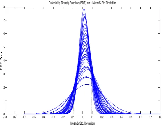
Figure 2. Normal probability distribution with respect to the mean value and the standard deviation of a data for 38 questions.

-0.80 -0.7 -0.6 -0.5 -0.4 -0.3 -0.2 -0.1 0 0.1 0.2 0.3 0.4 0.5 0.6 0.7 0.8 1

2 3 4 5 6 7 8

Mean & Std. Deviation

P

D

F

P

(x

i)

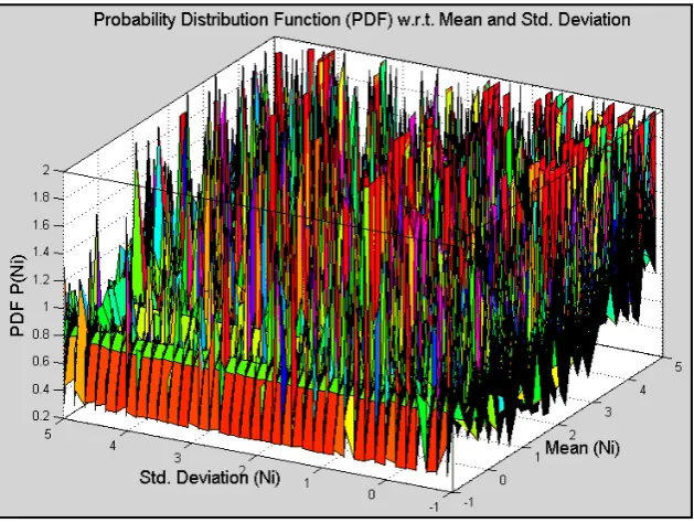
Figure 3. Normal probability distribution with respect to the mean and the standard deviation of data set for chosen 38 questions.

As depict in the figure 2, there are 38 different curves, showing the normal probability distribution curve for every question and thereby we see that an arbitrary data point belongs to the considered data sample. Such a generation to an extent affects the mean (𝑥𝑥̅= 0) of the data and offers only the variability about the average value and thus renders the possibility to minimize the undermining mistakes at a given stage of the evaluation. Moreover, it appears constructive to multiply the values of the Type A estimated standard deviations and Type B standard deviations by an appropriate sensitivity coefficients in order to bring them in the same units as the measure and thus we may take an account of concerned factors in the functional relationship between the input quantities and the output quantities of a given experiment.

Accordingly, in the figure 2 & figure 3, the probability distribution 𝑃𝑃(𝑥𝑥𝑖𝑖) with respect to the mean 𝒙𝒙� and the standard deviation 𝜎𝜎 show how the probability distribution is varying about the classical behavior of uniform system and how the errors are varying for the chosen data. Moreover, in both the above figures 2 & 3, the 𝑃𝑃(𝑥𝑥𝑖𝑖) with respect to mean and the standard deviation 𝜎𝜎 give general ideas in order to render prediction of the uncertainty varying over a given set of the data. Note that for a large sample size it is enough to estimate the probability distribution, see for the meshgrid consideration in the figure 3, where all the peaks are showing expected true values with respect to the mean 𝑥𝑥̅ and the standard deviation 𝜎𝜎.

During the above analysis, we find that the absence of a countable number of uncertainties lead to a proper normal probability distribution. The identification of sources of the uncertainties is the most important part of the process. Quantification of uncertainties in testing the normality involves a large element of estimations of Type B uncertainty components. As a result, it is rarely acceptable to

apply unnecessary endeavors in attempting specific assessment of uncertainties concerning the testing purpose.

All values of 𝑥𝑥̅ falling between 𝑥𝑥̅ − 𝜎𝜎 and 𝑥𝑥̅+𝜎𝜎 yield an equally likely distribution of the uncertainties, which may thus be significant towards the interpretation of the results of the test; for example, we may seek such a procedure in deciding whether a specific value is or is not. Numerical value in question is modeled by a normal probability distribution; there are no finite limits that will contain 100% of its possible value. However, for an example, ±𝜇𝜇(3) standard deviations 𝜎𝜎 are, regarding the mean of a normal distribution observe 99.73% limits. Thus, if the limits 𝜎𝜎- and

𝜎𝜎+ of a normally distributed quantity with mean (𝜎𝜎+ - 𝜎𝜎-)/2

are considered to contain "almost all" of the possible values of the chosen quantity, that is, approximately 99.73% of them, hence in this case, the standard uncertainty (µ)is approximately reduces to 𝜎𝜎/3, where 𝜎𝜎= (𝜎𝜎+ −𝜎𝜎−)/ 2 is the half-width of the underlying interval. In the figures 2, the 𝑥𝑥̅is the expectation or the mean of the distribution, and lies between the dotted line region representing ±0.09 of the average standard uncertainty (µ), which is taken about the mean value. For a normal distribution, the quantity ±𝜇𝜇

encompasses a definite range between the true probabilities, for instance 7.97% of the reported distributions.

Moreover, we observe further that the two simulated quantities are always nearly the same, and are close to the true probabilities. From the above discussion, if we know that the

𝑥𝑥

, and

𝑥𝑥̅

remains unknown, then the unknown

𝑥𝑥̅

renders to have a 0.0797 probability lying in the range of

𝑥𝑥̅ − 𝜎𝜎 and 𝑥𝑥̅+𝜎𝜎. That is with about 8% confident, we find that the unknown

𝑥𝑥̅

lies between 𝑥𝑥̅ − 𝜎𝜎 and 𝑥𝑥̅+𝜎𝜎. Underlining that 𝑥𝑥̅ − 𝜎𝜎 and 𝑥𝑥̅+𝜎𝜎 are “random interval”, the 𝑥𝑥 is a randomly drained observation from the population and is thus it may be viewed as a random variable set { 𝑥𝑥� − 𝜎𝜎,

[image:5.595.148.463.75.312.2]

3.1. Comparative Analysis

Data used for the comparative analysis of our results are reported in Ref. [25] and associated detail can be found online at the website:

(http://research.dfci.harvard.edu/Korsmeyer/MLL.htm). In this particular analysis, the chosen leukemia data set contains large genes samples (namely 12582 genes and 37 questions including 20 ALL & 17 AML). For examining the universality of our model and its similarity with an experimental data set as used in Ref. [24], we select only the samples that are the part of the training set [25]. Subsequently, by following an equivalent procedure for the data preparation as we performed earlier for the data set of [24], we find that the data set of [25] is large enough and it includes extraordinarily less data gaps and thus it renders an excellent analysis for the prediction purpose. After normalization, the experimental values of every question lies within a very narrow range from -1.2 to 4.5, which is the basis for small error and thus an accurate prediction of the uncertainties. Reported results are given in Table 2. Namely, the Table 2 shows error and uncertainty in the new data of

[25], wherefore we find it consistence and similar to the previous analysis carried forward from [24]. Since new reported data gives consistent behavior in large, avoiding chopping of the samples. As a result, as shown by dotted line reason in the figure 4, this prediction includes a variability of ±0.3 of the average standard uncertainty (µ) from the origin(𝑥𝑥̅= 0). The total probability distribution are showing in figure 4 and figure 5 (PDF in meshgrid, rendering all the expected peaks at true values with respect to both the 𝑥𝑥̅ and σ. It gives an excellent normal probability distribution, showing the equally likely distribution alike in the initial study of leukemia. In this case, the normal distribution, for a given average standard uncertainty ±µ, comprises a confident rage between the true probabilities, viz. 23.58% of the reported distribution, see figure 4.

[image:6.595.123.489.363.673.2]

Finally, it is shown that the combination of the average standard deviation gives an excellent approximation to the normal distribution. Herefore, the fundamental statistical method of estimating uncertainties enable us to explain the study of cancer data and general natural data sets. Such a proposition can indeed be applied to new biological sensitive data towards the modeling purpose of an invitro.

Table 2. Reporting statistical values of uncertainty predictions for the comparison with leukemia data set [25].

Mean (𝑥𝑥̅) Deviation Std. (σ)

Average Linear error(∆𝑥𝑥̅)

Standard Error of Mean

(SME) RMSE

min max average min max - min max average min max average

0.07 0.13 0.10 0.25 0.34 2.0E-13 _E-03 2.2 _{E-03 2.6E-03} 3.1 _E-15 2.8 _{E-14 2.5E-14} 8.4

Figure 4. Normal probability distribution with respect to the mean value and the standard deviation of a data for 37 questions [25].

-1.3 -1.2 -1.1 -1 -0.9 -0.8 -0.7 -0.6 -0.5 -0.4 -0.3 -0.2 -0.1 0 0.1 0.2 0.3 0.4 0.5 0.6 0.7 0.8 0.9 1 1.1 1.2 1.30 0.2

0.4 0.6 0.8 1 1.2 1.4 1.6

Mean & Std. Deviation

PD

F P(

x

i)

Figure 5. Normal probability distribution with respect to the mean and the standard deviation of data set for chosen 37 questions [25].

4. Conclusion

In this paper, we have discussed various fundamental causes concerning both the uncertainty and variability present in due course of the risk assessment of hazards to human health. We have concentrated on hazard depictions and associated effect in order to obtain information concerning the composition, and risk characterization, which can be helpful in developing a predictive model for the assessment of present risk in a given data set. Hereby, we have offered a precise consideration and underlying statistical reasons behind the uncertainty and variability in the risk assessment and management policies towards the regulatory purposes.

In this study, we explore statistical investigation concerning the error and uncertainties occurring in every measurement, even result of such measurements are taken carefully and it is unfeasible to remove the errors occurred in a particular measurement. So that, the analysis reported the mean 𝑥𝑥̅, standard deviation 𝜎𝜎 for every question 𝑁𝑁𝑖𝑖, and average linear error ∆𝑥𝑥̅, average standard error of the mean (SME) and the average root mean square error (RMSE) of a complete data set.

In this concern, the figure 2&3 depict every detailed analysis of the normal probability distribution with respect to a test mean value and standard deviation for such a data set. This helps us in making a clear understanding about the uncertain region of a data set. Namely, in this study, we find an average uncertainty of ± 0.09 (σ), where the lower and upper ranges lie between the true probability 7.97%, rendering a confidence level of the population mean falling between an interval around the samples mean, as it is identified in our present proposal. Moreover, for the leukemia data set reported in Ref. [25], we have offered a

comparative analysis in order to demonstrate the significance of the present statistical modeling.

In brief, the uncertainty is a quantitative estimation of errors present in a given data, where all the underlying measurements contain a definite uncertainty generated through systematic errors and/ or random errors. Hereby, acknowledging the uncertainty of a data is an important component while reporting the results of a given scientific investigation. Moreover, the undermining uncertainties are commonly understood to mean that one is less certain of the results, although the reported methodology of a subsequent analysis specifies the degree of uncertainties in a given experimental data and the final outcomes. This offers a confidence in novel statistical and scientific data explorations. Such a careful methodology can in principle reduce uncertainties by correcting the underlying systematic errors and minimizing the random errors. However, by the means of uncertainty analysis, it is difficult to reach to a zero error sample. We leave these issues open for a future study, concerning the statistical data samples and an optimization of the limiting data sample.

REFERENCES

[1] NIST SEMATECH, e-Handbook of Statistical Methods,

2012, Online available from http://www.itl.nist.gov/div898/handbook/.

[2] E. Smith, Uncertainty Analysis, Encyclopedia of

Environmetrics, John Wiley & Sons, Ltd, Chichester, Vol. 4, 2283-2297, 2002, ISBN: 0471 899976.

[image:7.595.140.467.74.319.2]

[4] K. Pearson (b), Statistical Tests,Nature, Vol.136, 550, 1935. [5] R.S. Fisher, Statistical Methods and Scientific Inference,

Hafner Press, New York, 1973.

[6] W. Heisenberg, Überden anschaulichen Inhalt der

quantentheoretischen Kinematik und Mechanik, Z. Phys., Vol.43,No.3–4,172-198,1927.

[7] B. N. Tiwari, On Generalized Uncertainty Principle, LAP Lambert Academic Publishing, Germany, 2011, ISBN-978-3-8465-1532-7.

[8] M. K. Beard, B. P. Buttenfield, S. B. Clapham, NCGIA Research Initiative 7: Visualization of Spatial Data Quality. Technical Paper 91-26, National Center for Geographic Information and Analysis. ftp: ncgia.ucsb.edu. 59.

[9] L. Kirkup, R.B. Frenkel, An Introduction to Uncertainty in Measurement Using the GUM (Guide to the Expression of Uncertainty in Measurement), Cambridge University Press, Cambridge, U.K., 2006.

[10] A. Kallner, Attending Physician Must Consider Uncertainty. Don't let yourself be cheated by the numbers!, Lakartidningen, Vol.103,No.35,2467-2469,2006.

[11] GUM 1993, Joint Committee for Guides in Metrology (2011). JCGM 102: Evaluation of Measurement Data - Supplement 2 to the "Guide to the Expression of Uncertainty in Measurement" - Extension to Any Number of Output Quantities. JCGM. Retrieved 13 February 2013.

[12] L. J. Gleser, Assessing Uncertainty in Measurement, Statist. Sci., Vol.13, No.3, 277-290, 1998.

[13] J. Ma, R. R. Wilcox, Robust Within Groups Anova: Dealing With Missing Values, Mathematics and Statistics, Horizon Research Publishing, Vol.1, No.1, 1-4, 2013.

[14] M. F. Goodchild, B. P. Buttenfield, J. Wood, Introduction to Visualizing Data Validity, In H.M. Hearnshaw and D.J. Unwin, editors, Visualization in GIS. New York: Wiley, 141–149, 1994.

[15] K. Brodlie, R. A. Osorio, A. Lopes, A Review of Uncertainty in Data Visualization, Expanding the Frontiers of Visual Analytics and Visualization, Springer London, 81-109, 2012, 978-1-4471-2804-5.

[16] R. Guo, Y. Cui, D. Guo, Uncertainty Statistics, Journal of Uncertain Systems, Vol.6,No.3,163-185, 2012.

[17] C. Srivastava, Support vector data description, LAP Lambert Academic Publishing, Germany, 2011, ISBN-13: 978-3844385212.

[18] K. M. Krishna, P. K. Kalra, Detection, Tracking and Avoidance of Multiple Dynamic Objects, journal of Intelligent and Robotic Systems, Vol.33,371-408, 2002. [19] C. Srivastava, Clustering and Neural Network Approaches for

General NN-Simulator, LAP Lambert Academic Publishing, Germany, ISBN 978-3-8454-0942-9.

[20] C. Srivastava, Face Localization, Color Images and Postural Degradation, LAP Lambert Academic Publishing, Germany, 2011, ISBN 978-3-8454-2889-5.

[21] C. Holzhüter, A. Lex, D. Schmalstieg, H. J. Schulz, H. Schumann, M. Streit, Visualizing Uncertainty in Biological Expression Data, Proc. SPIE 8294, Visualization and Data Analysis, Vol.8294,1-14,2012.

[22] R. N. Germain, M. M. Schellersheim, A. N. Lazar, I.D.C. Fraser, Systems Biology in Immunology: A Computational Modeling Perspective, Annual Review of Immunology Vol. 29, 527-585, 2011.

[23] K. Alden, M. Read, J. Timmis, P. S. Andrews, H. V. Fernandes, M. Coles, Spartan: A Comprehensive Tool for Understanding Uncertainty in Simulations of Biological Systems, PLoS Comput Biol, Vol. 9, No.2, 2013.

[24] T. R. Golub, D. K. Slonim, P. Tamayo, C. Huard, M.

Gaasenbeek, J. P. Mesirov, H. Coller, M. L. Loh, J. R. Downing, M. A. Caligiuri, C. D. BloomÞeld, E. S. Lander, Molecular Classification of Cancer: Class Discovery and Class Prediction by Gene Expression Monitoring, Report: Science, Vol.286, 1999, Online available from www.science.org.