Rain Fed Sorghum (Sorghum bicolor L. Moench) Crop
Growth Yield Forecasting Model
Adil Bashir Karrar
1, Hassan Ibrahim Mohamed
2, Haitham Ragab Elramlwai
3, Atif Elsadig Idris
4,*1Department of Agric. Engineering, Faculty of Engineering, University of Sinnar, Sudan
2Department of Agric. Engineering, College of Agricultural Studies, Sudan University of Science and Technology, Shambat, Khartoum
North, Sudan
3Centre of Dry Land Farming Research and Studies, University of Gadarif, Sudan
4Department of Agronomy, College of Agricultural Studies, Sudan University of Science and Technology, Shambat, P.O. Box 71,
Khartoum North, Sudan
*Corresponding Author: atifelsadig@yahoo.com
Copyright © 2014Horizon Research Publishing All rights reserved
Abstract
Agricultural production in Sudan is largely rainfed. For most Sudanese people sorghum is the staple food and its production is critical for national food security. Crop forecasting is the art of predicting crop yields and amounts of production before the harvest actually takes place, typically couple of months in advance. Several techniques can be used for crop forecasting. Crop forecasting relies on computer programs that describe the plant-environment interactions in quantitative terms. Such programs are called models. A twin-track approach was adopted, in which the fieldwork was linked to computer modeling. The outcome of the modeling effort was the development of the crop growth and water productivity prediction model. The model is a deterministic, process-based physical model with daily time-step cropping systems. The model can simulate the soil-plant water budget, crop canopy and root growth, and dry matter production for Sorghum crop. Experiments were done at Sinnar, AbuNa'ama and Gedaref areas during the same season. A simple, two layered soil, water balance model is used, based upon assumptions that the soil has a moderate hydraulic conductivity and no drainage impediment, there is no storage of water in excess of field capacity beyond one day, the water table is deep and there is no significant contribution from groundwater, the water content of the root zone is uniformly distributed at the end of each day, model takes no direct account of soil fertility, technology (mechanization, fertilizer use), varietal differences and farming practices. Inputs are daily date since sowing, mean or average daily temperature in degree Celsius, daily pan evaporation (mm), daily rainfall (mm), which is the only source of infiltration into the soil. Sorghum grain yield is estimated by the model as the main output. The ability of the model to provide reasonable estimate of rain-fed sorghum yield according to Chi square test is reasonable, and therefore, the model can be used for forecasting sorghum yield in the study area.Keywords
Simulation Model, Sorghum Crop Growth, Rain Fed Agriculture, Rain Water Productivity1. Introduction
Agricultural production in Sudan is largely rain-fed. For most Sudanese people sorghum is the staple food and its production is critical for national food security. Crop forecasting is the art of predicting crop yields and amounts of production before the harvest actually takes place, typically couple of months in advance. Several techniques can be used for crop forecasting. Crop forecasting relies on computer programs that describe the plant-environment interactions in quantitative terms. Such programs are called models. They attempt to simulate the plant-weather-soil interactions, and they therefore need information and data on the most important factors that affect crop yields. National planners are giving increasing importance to the monitoring of crops and the assessment of final production in terms of dependence on weather conditions. In developing countries production increase has been much slower, while there is a drastic increase in the population due to improved living conditions. As a result it is very necessary to forecast size and quality of harvests, particularly cereal crops. Some countries conduct rapid estimates based on interviews with farmers. Other countries have developed biometric systems based on measured crop indices (plant density, maize cob size). In some countries agricultural statistics are so uncertain that the agro-meteorological forecasts are taken as final yield and production figures. The agro-meteorological approach usually gives best results in semi-arid areas where the water deficit is the main limiting factor. Simple statistical or trend models perform very poorly in semi-arid countries, where the inter-annual variability of yields reaches very high values. Best results can be obtained with relatively simple simulation models where more emphasis was given to the accurate selection of value added agro-meteorological variables than to the processing of large volumes of input data.
encounter great difficulty in producing accurate crop yield and production estimates; mainly due to poor organization of statistical services, in addition to the fact that results are assembled too late to provide adequate information for early warning and emergency food procurement.
Rainfed semi-mechanized farming system in Sudan was developed under the auspices of the government as mechanized crop production schemes in 1945. The area under this system of management increased rapidly and by the beginning of the 1970s was estimated to have reached 840000 hectares. It has spread to about 5880000 hectares in the states of El Gedaref, Blue Nile, White Nile, Sinnar, and Southern Kordofan (Nuba Mountains) (Fig. 1).
Sorghum is the dominant summer cereal crop in Sudan, where more than 80% of the area is grown under rainfed conditions. Most of the sorghum area lies in the central clay plain, which is confined between 450 mm and 600 mm rainfall isohyets. Sorghum is grown as a multi-purpose crop, the grain being used for human consumption and the straw serves for animal feeding, as building material, fire wood and for various other local purposes.
Simulation is defined as reproducing the essence of a system without reproducing the system itself. In simulation the essential characteristics of the system are reproduced in a model, which is then studied in an abbreviated time scale. Simulation techniques are increasingly used to support field research. A model is a schematic representation of the conception of a system or an act of mimicry or a set of equations, which represents the behavior of a system. Its purpose is usually to aid in explaining, understanding, or improving performance of a system. A model is, by definition a simplified version of a part of reality, not a one to one copy. This simplification makes models useful because it offers a comprehensive description of a problem situation. However, the simplification is, at the same time, the greatest drawback of the process. Input variables are those which characterize external action on the system, they include essentially the weather and management. Outputs are simply the variables which the user decides to look at. Some of them will be used for model verification and validation, others, like yield, are of immediate practical relevance.
Crop models pose distinct advantages for use in scientific research. Traditional infield research requires significant investments of time, labor, money, and other resources. Cropping systems research usually requires long-term experiments to take into account variations in yearly climatic conditions, such as temperature and precipitation. Crop models, once calibrated, allow researchers to simulate multiple years of experiments, utilizing historical weather data, in a matter of hours. [1] used CERES-Wheat and CERES-sorghum to simulate a wheat-sorghum-fallow and wheat-fallow rotations and successfully showed that crop models could be used as dryland cropping systems research tools. Also [2] used RAINBOW, COROPWAT, and CROP BUDGET software’s under different scenarios of rainfall levels and distribution to simulate sorghum. They found them to be capable to fairly predict crop yield at various
levels of soil moisture.
[3] stated that when in the early 1980s desktop computers became powerful enough to carry out most engineering design, many large design organizations developed their own canal design software using a programming language such as FORTRAN or Basic. But by the mid 1990s spreadsheets had become so sophisticated that they could handle most situations arising in the design of irrigation projects. The advantage of spreadsheets is their replication capability by copying rows, and 'what-if' capability. Any variable can be changed and its effect on other parameters can be seen immediately. They also have the added advantage that all data are visible, graphical checking is easy, and data can be imported or exported easily to feed into other software such as CAD or surveying packages. Since they are used almost universally for all manner of calculations, every engineer in a computer-literate environment understands their use. The great power of a spreadsheet stems from its copy function. the of this study was developed using Excel spreadsheets.
As [5] stated it is stressed that, according to the scope of the model i.e. research, training, management or planning tool, the input data may vary. In general management applications of crop simulation models can be defined as:
1) Strategic applications where crop models are run prior to planting.
2) Practical applications crop models are run prior to and during crop growth.
3) Forecasting applications models are run to predict yield both prior to and during crop growth [6].
[6] concluded that various kinds of models such as statistical, mechanistic, deterministic, stochastic, dynamic and static simulations are in use for assessing and predicting crop growth and yield. Crop growth model is a very effective tool for predicting possible impacts of climatic change on crop growth and yield. As stated by [5] crop-yield weather modeling refers to the techniques which can be used operationally to determine the likely effect of weather on yields. As cited by [7] many computer simulation models of plant growth have been documented in the literature [8-14]. These physiologically based models require extensive meteorological, management, and soil inputs with varying degrees of accuracy in order to model crop growth. [15] concluded that ZIMsched (a spreadsheet based model) is a robust, scientifically sound and yet simple irrigation management and yield forecasting tool. It has been developed in Zimbabwe but should have wide application with minor, if any, modifications. As stated by [16] that because a model is a simpler representation of a real system, it is actually an incomplete or imperfect description of the system. There is always some loss of information when a real system is translated into a model. A model does not tell us the whole picture of the system, only the essential parts that are important to explain the system’s behavior, function and purpose. This incomplete depiction of a system means that the estimations or simulations from a mathematical model are subject to error.
of water content in the rooted soil, at consecutive time periods. The soil water balance approach has been used in a lot of papers; either explicitly or included in simulation models [17, 18, 19]
[5] stated that phenology qualitatively describes the successive stages in the development of plants, from seed germination to flowering to maturity. Since the stages are very plant dependent, it is difficult to define a universal system to describe phases, as only the main stages (germination, differentiation of flowers, flowering, seed formation, seed filling, and maturity) are common to almost all flowering plants. All models include a phenology component. Temperature plays a very directly observable effect on the rate of development of plants and cold blooded organisms. The most common method to determine the effect of temperature is the often criticized method of temperature sums, also known as Sum of Degree-Days (SDD), or thermal time (GDD). The method assumes that the amount of heat (measured by temperature) required for a plant to develop from planting to the seed formation stage is constant. Starting from planting, the following sum is computed:
SDDs =�Day on which stage S is reachedPlanting day (T − Tb) (1) T- Tb is taken as 0 when T< Tb
T is taken as Tu when T> Tu
where: T is average daily temperature, Tb is the base temperature below which no development takes place, and Tu is an upper threshold temperature above which it is assumed that temperatures ceases to have an effect on development.
As [20] cited CERES-Sorghum is a daily time-step model that predicts grain sorghum yield, phenology, yield components, biomass, root growth, soil water balance, and soil nitrogen balance. [21] stated that for most crops, temperature is the primary driving factor controlling phenology, although many other factors can be important including photoperiod, water, nutrients, carbon dioxide, and salinity. The phenology sub-model uses thermal time i.e., GDD as an input parameter for each species, to simulate the time from sowing to maturity, with no adjustment for other factors known to impact development. [22] stated that in CropSyst, phenology is determined by thermal time, i.e. a specific development stage is reached when the required daily accumulation of average air temperature above a base temperature and below a cutoff temperature is reached.
1.1. Methods of Yield Prediction
[4] presents three modeling methods namely; descriptive, regression and crop simulation methods. Descriptive methods simply classify weather conditions according to one or several variables to identify conventional threshold separating groups of significantly different yields. Regression methods derive equations relating crop yield with weather variables. While, simulation methods which
are the most complex ones currently in use, analytically describe the physical and physiological impact of the environment and management conditions on crop development, growth and yield. [4] stated that a model run it simulates yield of the plant-environment-management system for one set of model variables, environmental variables and management inputs (i.e. only a limited number of situations which could apply to one very specific field). In addition the objective of agro-meteorological crop yield forecasts is to estimate yield at regional level, several techniques must be applied to convert the yield output by a model to regional averages. He concluded that agro-meteorological crop yield forecasting approaches differ widely in terms of input data requirements and model complexity, resulting in very variable robustness, development, and implementation costs.
[23] reported that to be able to forecast yields from a fairly simple database, there are essentially two requirements, a forecasting algorithm, and a model that can be used with this algorithm and the available data to enable reliable forecasts of crop yield to be made. As stated by [24] one of the more useful and widely accepted production function forms is based on the consumptive use, or evapotranspiration (ET) of water, as a yield index. [25] reported that the evapotranspiration production function (Etpf) in Farmington measured using a sprinkler line source and the water balance equation and assuming drainage was zero was linear as reported in the literature for most Etpf functions:
Y = -37393.8 + (1358.302*ET) R2 = 0.96. (2)
Where: Y is yield (kg ha-1). ET is evapotranspiration (cm).
For Las Cruces the function with sprinkler system is linear and can be given by:
Y = -35300 + 1224.2*X R2= 0.97 (3)
Where: Y is yield (kg ha-1). X is the ET (evapotranspiration
in cm).
The measured water production function (water applied versus yield) obtained at Las Cruces, using a drip irrigation system is curvilinear in nature. The function is computed using a second order polynomial as:
Y = -7809.28 + 693X – 1.164X2 R2 = 0.90 (4)
Where: Y is the yield (kg ha-1). X is the water applied
including rainfall (cm).
different spatial and temporal (daily, weekly, seasonal, yearly) scales [26]. In agronomic terms, water use efficiency is defined as the amount of organic matter produced by a plant divided by the amount of water used by the plant in producing it [27]. This definition relates both production and utilization of water resources in agricultural production systems. [28] expressed WUE as grain yield per unit ET.
[29] stated that water use efficiency of different crops was determined by dividing the grain yield by the water used (sum of soil water at planting- soil water at harvest + irrigation water + effective rainfall) expressed as kg/ha.mm-1. The soil upward flux was negligible because of
deep ground water table (>3.0 m). However, the used terminology water use efficiency does not follow the classical concept of efficiency, which uses the same units for input and output. The classical concept of efficiency as used by engineers omits production values. International Water Management Institute (IWMI), therefore, has proposed a change of the nomenclature from water use efficiency to water productivity. The productivity per unit water in the irrigated sector and the labor productivity in Sudan exhibit low productivity for both water and labor resources and particularly for the rain-fed crops.
Runoff occurs when the surface water depth is greater than the surface storage. Runoff co-efficient, the ratio of the maximum rate of runoff to the uniform rate of rainfall with a duration equaling to, or exceeding the time of concentration which produced this rate of runoff. The amount of runoff is usually expressed as a percentage of the total rainfall in a given area. The Soil Conservation Service of USA (SCS) runoff curve number method has been employed for computing runoff depth to assess water harvesting potential in the region. According to [31] the simplest method for estimating daily runoff is the linear regression of daily rainfall to daily runoff. However, this method sometimes leads to excessive errors in the estimated runoff because soil characteristics are ignored. Another simple type of runoff model is referred to as the infiltration index (F index). This model has been used to estimate the daily amount of runoff under specific soil and climate conditions [30, 32] give the threshold linear model of daily rainfall (RF) and runoff (RO) processes (mm/day) for the CT production technique (PutuRO), as follows:
RO = 0 if RF <15 (5)
RO = 0.05*RF if 15<RF ≤ 25 (6)
RO = 0.1*RF if 25<RF ≥ 50 (7)
RO = 0.2*RF if RF>50 (8)
As given by Schwab et al. (1971) runoff rate (m3/s) by using the rational formula: Q=0.0029*C*I*A (9) Where:
C = runoff constant. I = rain intensity mm/hr.
A = area in hectare.
According to [34] runoff may be estimated using the expression developed by the USDA Soil Conservation Service [35] proposed to estimate runoff from rainfall to be 75% of incoming rainfall.
1.2. Models Validation, Calibration and Sensitivity Analysis
It was cited by [5] that before models can be put to work in assisting with decisions in the real-world, the user must be reasonably confident that the model describes actual crop responses to weather and management with a degree of precision that is sufficient for the intended application. The standard wording usually resorted to in this context includes validation, calibration, verification, etc., but there is no consensus in their actual acceptation. Some terms, like accuracy, appear to be used only in particular contexts such as crop forecasting. In fact, maybe with the exception of evaluation, the meaning of some of the words varies according to the type of model, and the concepts themselves have a subjective element.
Validation is more difficult. There is no such thing as a definitive or final validation of a model. A model must be validated at the same spatial scale and with the same type of data as those that will be available in operational work. In other words, validation is the sequence of tests and checks that convince the user that the model is valid for the intended purpose. If a model has been validated for many different circumstances, the potential user can decide that it may perform properly even under his own conditions, but he should not take it for granted.
It was stated that there is no single statistical analysis appropriate for assessing the performance of deterministic simulation models [36, 37]. The choices are currently limited to somewhat simplistic analyses based upon either regression or goodness-of-fit tests [40]. The validation can be applied using regression analyses of the form (Y = a + b*x) fitted by Genstat 5 [38] between individual sets of simulated (Y) and observed (X) data. The regression coefficients measure the degree of bias of the simulation and in this form allows under- or over-estimation behavior to be identified. When (a) is not different from zero and (b) is not different from unity, no bias is indicated. Assuming that the author or the user of a model is satisfied with the algorithms, the next step is to submit the model to the ordeal by real-world data: the model is run repeatedly with actual inputs to see if it mimics reality sufficiently well. The actual data are usually referred to as calibration data or training data. The greater the variety of training data, the greater the chances that the model will behave under new conditions. Needless to say, if next to statistical and physiological criteria we also adopt agronomic criteria and constraints, like using the model at a different geographic scale than the one for which it was developed, the best parameters may still be different.
changes in the input data and in the model parameters. This covers several different techniques. The simplest is to plot the values of a selected output variable against a range of values of an input variable or a parameter. The shape of the resulting functional relationship is interesting in itself (linear, maximum, minimum, constant), and should makes sense from a physiological and agronomic point of view. It will appear, in many cases that the effect of one single parameter is relatively limited. In crop forecasting, sensitivity analysis is often used to see the effect of the parameters on the errors affecting the forecasts. A convenient way to approach sensitivity analysis is to plot the both the output variable O and the input parameters P of interest as a percentage of their normal ranges: this immediately indicates the effective role of the parameter and the fact that other factors are at work.
In this study a method was developed to assess crop yield depending on daily climatic conditions; in addition to the assessment of dry matter and water use efficiency. This study was conducted with the aim of providing an understanding of the use of modeling to predict growth and yield. To develop, verify and apply a computer model to predict yield, dry matter, water use efficiency (WUE), precipitation use efficiency (PE) and runoff losses from rainfed farming techniques.
2. Materials and Methods
Experiments were done at Sinnar, AbuNa'ama and Gedaref areas during the same season. In these areas rains usually commence in May with relatively light showers but the effective rainy season starts in late June, increases in July, and reaches its peak in August (Figure, 4). The rainy season is characterized by extreme variability in annual amounts and distribution within each season. There is also a wide variation in frequency, intensity, and duration of individual events.
AbuNa'ama area: lies about 400 km south of Khartoum. Mean monthly temperature ranges (Figure, 2) from a mean maximum of 40°c to a mean minimum of 21.1°c during the rainy season (from June to October) according to ClimWat software of the FAO. experiment was conducted on a clay soil classified as a vertisol, at Faculty of Agriculture, University of Sinnar; top farm.
Sinnar area: lies about 300 km to the south of Khartoum. Mean monthly temperature ranges(Figure, 2) from a mean maximum of 41.1°c to a mean minimum of 21.5°c during the rainy season (from June to October) according to ClimWat software of the FAO. The experiment was conducted on a clay soil classified as a vertisol, at the Islamic Development Company for Agricultural Services site.
Gedaref area: lies about 300 km to the south of Khartoum. Mean monthly temperature ranges (Figure, 2) from a mean maximum of 37.5°c to a mean minimum of 22.4°c during the rainy season (from June to October) according to
ClimWat software of the FAO. The experiment was conducted on a clay soil classified as a vertisol, Demonstration Farm of the Faculty of Agricultural and Environmental Sciences, University of Gedaref at Twawa area.
The effect of these high maximum temperatures during the growing season is reflected by high evapotranspiration rates (Figure, 3) resulting in great losses of the stored moisture within the soil which quickly dries up and hardened.
Relative humidity is directly influenced by rainfall. During the rainy season the average relative humidity ranges from 40-80%. With cessation of rains it falls sharply and remains in the range of 15-25% throughout the dry season.
The topography of the study areas is generally flat, with a mild slope from west to east. Soil of the study area is predominantly Vertisols, deep dark colored clays of montmorillonitic mineralogical origin (clay content is 40-65%). Vertisols are characterized by very low permeability and hydraulic conductivity when wet. These characters impede infiltration of rain water and consequently the ability of soil to store water. In addition, the readily available soil moisture (max. allowed depletion% *(field capacity - permanent wilting point) is quite low relative to the total soil moisture content (Figures 5 and 6). This may result in crop water stress as the moisture content approaches the wilting point [39] Cracks develop when the soil dries up by the end the rainy season. Early rains penetrated into the soil through these cracks before they closed. Runoff usually occurs when high showers follow heavy rains.
The approximate plot dimension was 10 m by 5 m with 2 m as border areas between adjacent plots. The land was cleared from shrubs. Land preparation was done using wide level disc, the conventional machine. Sorghum, (Sorghum bicolor L. Moench); variety Arfa’a gadamak was planted at the recommended seed rate. Weeds were controlled as necessary using hand pulling and hand tools.
2.1. Data Collection
Daily agro-meteorological data namely rainfall, pan evaporation, and mean temperature were collected from nearby meteorological stations in year 2006 for the expected rainy months.
measured at periods of ten days in both locations.
θw% = (Ww-Dw) ∗100/ Dw (10)
θv% = θw% * ρb/ρw (11) D = θv% * 200/ 100 (12) Where:
ρb: soil bulk density (gm/cm3),
D: soil moisture content in depth basis (mm), Ww: wet sample weight (gm),
Dw: dry sample weight (gm),
θw%: soil moisture content in gravimetric basis,
θv%: soil moisture content in volumetric base.
ρw: water density
At the end of the growing season, a 0.5 m * 0.5 m quadrant was thrown randomly over the growing plants in each plot. The grain yield per square meter was recorded and converted to kg/ha.
[image:6.595.64.291.431.744.2]Dry matter was determined at the end of the growing season, using a 0.5 m * 0.5 m quadrant thrown randomly over the growing plants in each plot. These plants were cut, tied in bundles and left to dry for 10 days under the sun, and then weighed to give the air-dry yield this is done at Sinnar site only.
Figure 1. model flow chart.
2.2. Development of Crop Growth and Water Productivity Prediction Model
2.2.1. Model Assumptions
A simple, two layered soil, water balance model is used, based upon the following assumptions:
1- The soil has a moderate hydraulic conductivity and no drainage impediment.
2- There is no temporary storage of water in excess of field capacity beyond one day.
3- The water table is deep and there is no significant contribution from groundwater to the root zone.
4- At the end of each day, the water content of the root zone is uniformly distributed.
5- Rainfall and irrigation systems do not apply water at such high application rates as to exceed the infiltration capacity of the soil.
6- The model takes no direct account of soil fertility, technology (mechanization, fertilizer use), varietal differences and farming practices.
The model flow chart is depicted in Fig. (1). 2.2.2. Inputs
Complex mechanistic water budgeting and crop growth algorithms, whilst theoretically attractive, are often of limited value in many practical applications because the data, information, and operator understanding they require are seldom available. Simpler and more robust algorithms have therefore been reviewed and incorporated into this model.
Table 1. model input parameters and their values.
Parameter value
FMAD 0.65
B.D. (1) 1.27 g/cm3
B.D. (2) 1.34 g/cm3
FC (1) W% 37
PWP (1) W % 22
FC (2) W % 37
PWP (2) W % 22
Surface Depression Storage 5 mm
Run_Off Coefficient 0.6
[image:6.595.311.552.456.635.2]Figure 2. Average daily temperature at the three sites during the growing season 2006/07.
G: Gedaref, ABU: AbuNa’ama and S: Sinnar.
Figure 3. daily pan evaporation at the three sites during the growing season 2006/07.
[image:7.595.58.303.259.405.2]G: Gedaref, ABU: AbuNa’ama and S: Sinnar.
Figure 4. daily rain at the three sites during the growing season 2006/07.
G: Gedaref, ABU: AbuNa’ama and S: Sinnar.
2.2.3. Model Requirements
Minimum system requirements to run the model are Processor Pentium 233 MHz or higher processor; Pentium III recommended. Operating system Microsoft Windows 2000 Service Pack 3 or later, or Windows XP or later (recommended); Memory 64 MB RAM (minimum); 128 MB RAM (recommended); Disk space 245 MB, including 115 MB of available space on the hard disk that contains the operating system. Hard-disk space usage varies
depending upon the configuration. A local installation source requires approximately 2 GB of hard-disk space during the installation; the local installation source that remains on users' computers requires as much as 240 MB of hard-disk space beyond that required for Office. Monitor Super VGA (800 x 600) or higher resolution with 256 colors. Disk drive required is CD-ROM drive. Pointing device is Microsoft Mouse, Microsoft IntelliMouse or compatible pointing device.
2.2.4. Model Process
The model was built up and developed using Microsoft Excel. It is a program that displays an electronic spreadsheet that allows user to do the operations of entering data, analyzing, and displaying the results in addition to graphical representations. It is used to calculate outputs from inputs using suitable formulae.
Table 2. Cumulative Growing Degree Units (F°) from Planting to Successive Growth Stages for Short and Long Season Grain Sorghum Hybrids
Growth Stage Short Season Cumulative GDUs (F°) Hybrid Full Season Hybrid
Emergence 200 200
3-leaf 500 500
4-leaf 575 575
5-leaf 660 660
Panicle Initiation 924 1365
Flag Leaf Visible 1287 1470
Boot 1683 1750
Heading 1749 1890
Flowering 1848 1995
Soft Dough 2211 2310
Hard Dough 2508 2765
Black Layer 2673 3360
Source: Sorghum Growth and Development, by Jason Kelly
The events of model processes include:
[image:7.595.312.552.319.569.2] [image:7.595.60.302.454.601.2]growing degree unit (GDU) system. GDU was calculated as (Jason Kelly ):
GDU = ((Daily max. air temp. + daily min. air temp)/2 )- base temperature (13) GDD's for every stage is in the table (2), it is given in degree Fahrenheit. In the model it is taken in degree Celsius.
2- Runoff using fixed coefficient of (0.6) as upper bound [41].
3- Deep percolation (DP) depends on water holding capacity of the soil layers and the amount of water coming from rain.
DP= RF-SW-RO (14) Where:
RF = rainfall amount.
SW = soil water holding capacity. RO = amount of runoff.
4- Leaf area index (LAI) using an equation that depends on degree day (DD) accumulation after [42] it is a power-exponential function. He calculated leaf area index for sugarcane crop without water stress (under irrigation), by regressions in which LAI and GDD were correlated:
LAI=e-13.521 *(∑GDD) 2.784 *e-0.004023*∑GDD
R2 = 0.58 (15)
In this model LAI is obtained using data from COROPWAT software for the sorghum crop.
5- Potential transpiration (Tpot) and potential evaporation (Epot) are function of LAI and daily pan evaporation (E), an input; after Ziaei and [43].The potential evaporation and transpiration are dependent on pan evaporation and leaf area index (LAI). The following equations are calibrated form of equations which were used by [23] which are based on the work of Tanner and Jury (1976):
Epot=Epan *exp (-0.55LAI) (16) Tpot=Epan *(1-exp (-0.55LAI)) (17) Where Epan is daily pan evaporation (mm), LAI is leaf area index (decimal), and Epot and Tpot are potential evaporation and transpiration (mm), respectively.
6- Actual evapotranspiration using formulas depending on potential evapotranspiration and soil moisture content, after [43]. The actual transpiration depends on location of available water in root zone and root activity. It is assumed that transpiration occurs at potential rate when available water is more than a specific fraction of holding capacity of soil layers. Otherwise, the actual transpiration (AT) decreases linearly to zero when the soil water content (SMC) is reduced to permanent wilting point (PWP).
Actual evaporation is calculated based on potential evaporation and the number of days from the last rainfall or irrigation as follows:
Eact=(Epot)*t -0.5 (18)
Where Eact is the actual evaporation, Epot the potential evaporation, and t is the number of days after wetting the soil. The total amount of transpired water is proportioned between soil layers corresponding to length of root in each layer. The total amount of removed water must be equal or less than potential transpiration. This process described by the following equations:
TLi=Tpot*(D+20)/DL (19) Where TLi is the transpiration from each layer, Tpot the potential transpiration, D the depth of root within the layer, and DL is the depth of layer. All values are measured in mm.
If Tli>Tpot then:
TLai=Tpot* TLi/∑TLi (20) Otherwise
TLai= TLi (21) Where, Tlai is actual transpired water from each layer. Both layers provide transpiration water unless one layer becomes dried or roots have been only extended to the first layer.
7- Transpiration efficiency (TE) is calculated using a formula that depends on daily pan evaporation (Epan), after [43, 44] and [23]. Following equation is used for computing transpiration efficiency as a function of daily pan evaporation, Epan in mm:
TE=102-13*(Epan)+0.53*(Epan)2 (22)
8- Root depth in different layers is given as daily root extension depending on 5-day pan evaporation by summing the previous five day pan evaporation data, and according to the soil moisture condition, after [43, 44, 23]. Following equations are used for downward extension of root:
DR(inc.)=11*1/5*EO0.5 (For dry conditions) (23)
DR(inc.)=9*1/5*EO0.5 (for wet conditions) (24)
Where EO is the 5-day pan evaporation, which is calculated by summing the previous 5 days of data, and DR(inc) is the daily root extension. The coefficients can be used as calibration variables. The dry and wet conditions are distinguished by the soil moisture limit which is used to distinguish between actual and potential transpiration.
9- Dry matter is given as a product of actual transpiration (AT) and transpiration efficiency (TE), after [43]
DM(inc.)= TE*AT (25) Where DM(inc.) is the dry matter increment (kg ha-1), TE the transpiration efficiency (kg ha-1 mm), and AT is the actual transpiration (mm).
Above ground biomass is given by:
AGB=0.8*DM(accu) (26) Where, ABG is the above ground biomass, and DM(accu) is the accumulated dry matter since sowing [43].
reported the following linear equation for sorghum: Y=0.58*(Above Ground Biomass)-1.26 R2=0.941 (27)
The above equation was calibrated and used in the model: Y= 0.0905*(Above Ground Biomass) +126.76 (28) 11- Water use efficiency was calculated as the grain yield (Kg/ha) divided by the total depth of water transpired (mm), after [29] and others.
12- Precipitation efficiency (PE) is grain yield (kg/ha) divided by the total seasonal precipitation (mm).
2.2.5. Models Outputs
The model process generates the following outputs:
Crop phenology, runoff losses, evapotranspiration (mm/day), dry matter (kg/ha), grain yield (kg/ha) and water and precipitation use efficiency.
3. Results and Discussions
The most important reason for model building is that experimentation with the structure and function of a model is more practical and economical than working with the actual field situation. Time and expense are the prime considerations here. Therefore the model is calibrated with actual data to improve its structure. In addition, it is used to attain its main function: forecast of yield and to generate various outputs under different scenarios of inputs to simulate practical cases and yield situations.
3.1. Yield Prediction
[image:9.595.312.556.227.353.2]The model is used to describe the development, growth, and determination of yield of rain-fed sorghum in the central clay plain of the Sudan. Its development and testing have focused on the semi-arid area of Sudan, but it may also find application elsewhere.
Table 3. predicted and observed sorghum yield (Kg/ha) and RMSE using the two methods.
Method Site Observed Yield (Kg/ha)
Estimated Yield (Kg/ha)
RMSE (Kg/ha)
Chi square
(χ2)
Model
Sinnar 790.24 842.53 89.78 3.25
AbuNa'ama 878.05 918.62 213.54 1.79 Gedaref 946.50 844.63 1351.12 12.28
Grain yield is estimated by the model as the main output, it is taken as a linear relationship with above ground biomass, and this relationship was after [46]. The simulated versus observed grain yield is shown in table (3), the estimated yield was 842.53 kg/ha at Sinnar site, while the observed yield was 752.75 kg/ha and the root mean square error (RMSE) was 89.78 kg/ha. At AbuNa'ama site the estimated yield was 918.62 kg/ha and observed yield was 604.67 kg/ha and the root mean square error (RMSE) was
213.54 kg/ha. Table (3) depicts the simulated and observed grain yield of these sites. The results of table (3) showed the ability of model to provide reasonable estimate of rain-fed sorghum yield according to Chi square test, and therefore, the model can be used for forecasting sorghum yield in the study area.
3.1.1. Soil Moisture Content (SMC)
Figures (5) and (6), depicts the simulated and measured soil water during the growing season for non-irrigation treatment against days after sowing. They are in a good agreement.
[image:9.595.315.553.384.499.2]Figure 5. Observed and simulated soil moisture content (Sinnar).
Figure 6. Observed and simulated soil moisture content (Abuna'ama)
3.2. Water and Precipitation Use Efficiency (WUE & PUE)
Water use efficiency (WUE) was calculated by the model as the ratio between grain yield and actually transpired water by plants at the end of the flowering stage (kg/ha.mm). Estimated WUE was 2.77 kg/ha.mm at Sinnar site; while the observed WUE was 2.42 kg/ha.mm and the root mean square error (RMSE) was 0.35. At AbuNa'ama site the estimated WUE was 2.81 kg/ha.mm; while the observed WUE was 1.99 kg/ha.mm and the root mean square error (RMSE) was 0.82. At Gedaref site the estimated WUE was 3.13 kg/ha.mm; while the observed WUE was 4.10 kg/ha.mm and the root mean square error (RMSE) was 0.98 (table 4).
[image:9.595.57.298.556.641.2]AbuNa'ama site compared to rainy days number (13 days) at Sinnar site, hence estimated evapotranspiration is higher at Sinnar site due to high temperatures.
Precipitation use efficiency (PUE) was calculated as the ratio between grain yield and precipitation through the growing period. At Sinnar site PUE was 2.89, at AbuNa'ama site was 2.01, and at Gedaref 2.16 (table 5.4).
This result was in agreement with [47,48], for Zea mays L. in Kenya and Burkina Faso.
3.3. Runoff Losses:
Runoff losses were estimated using a coefficient of (0.6)
(i.e. rainfall depth will be multiplied by this coefficient after subtracting a surface depression storage depth (SDS). The SDS was taken as (5 mm). Estimated runoff using this coefficient was similar to that estimated by the United States Soil Conservation Service method (SCS, 1972) using a curve number of 85 (average of the curve numbers that coincide with small grain land use and soil group D). This coefficient is stated by [26] At Sinnar site the estimated runoff was 142.3 mm out of 293.4 mm of rainfall, at AbuNa’ama site it was 204.8 mm out of 414.7 mm of rainfall and at Gedaref site it was 188.4 mm out of 406.6 mm of rainfall.
Table 4. water and precipitation use efficiency.
PARAMETER Est. yield (kg/ha) (TW) (mm) Total water Est. WUE Est. PUE Obs. Yield (kg/ha) Obs. PUE
SIN (site) 842.53 301.47 3.39 2.87 790.24 2.50
ABUN (site) 918.62 261.66 3.51 1.97 878.05 2.65
GEDAREF(site) 844.63 238.30 3.13 2.05 946.50 7.86
DRY (season) 827.24 295.76 2.80 3.42 790.24 2.55
NORMAL(season) 842.53 301.47 3.39 2.87 790.24 2.50
WET(season) 838.04 300.12 2.79 3.46 790.24 2.51
HEAVY (soil) 842.53 301.47 3.39 2.87 790.24 2.50
MODERATE(soil) 843.49 301.84 2.79 3.49 790.24 2.49
LIGHT(soil) 857.72 308.88 2.78 3.55 790.24 2.44
LOW (temp.) 1065.69 415.30 2.57 3.15 790.24 2.77
NORMAL (temp.) 842.53 301.47 2.79 3.48 790.24 2.50
HIGH (temp.) 731.39 238.10 3.07 3.72 790.24 2.31
EARLY (sowing) 913.57 376.27 2.43 3.78 790.24 2.00
MID (sowing) 863.17 326.63 2.64 3.73 790.24 2.30
LATE (sowing) 830.13 289.85 2.86 3.26 790.24 2.60
RUNOFF(0.6) 842.53 301.47 2.79 3.48 790.24 2.50
RUNOFF(0.4) 836.23 297.98 2.81 3.45 790.24 2.53
RUNOFF(0.2) 845.10 302.09 2.80 3.49 790.24 2.49
SDS(5 mm) 842.53 301.47 2.79 3.48 790.24 2.50
SDS(10mm) 824.61 292.71 2.82 3.41 790.24 2.57
SDS(15mm) 844.84 303.00 2.79 3.49 790.24 2.48
3.4. Model Verification
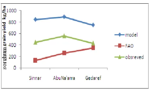
[image:10.595.63.549.247.672.2]Figure 7. Observed and model estimated yield.
Figure 8. Observed yield compared to model and FAO method estimated.
3.5. Model Validation
The root mean square of the residuals (RMSE) and adjusted coefficient of determination (R2) provides a
measure of the accuracy of the simulation. The RMSE is useful; it provides an absolute measure of overall error in the units of the simulated variables [44].
Validation of simulation models against independent data is an essential step in model development [19] It has, however, frequently not been possible to obtain suitably comprehensive data for validation even though great detail may have been available on individual aspects of crop response [40] In this work, the model of rainfed sorghum crop was constructed from published information after [43] and others, whereas the associated experimental program was designed to provide a comprehensive data set for model validation. Unfortunately, the phenological responses of the cultivar Arfaa Gadamak used in the experiments were not available. The model was build in an excel sheet using Sinnar site data and applied to AbuNa'ama and Gedaref sites data. The application revealed that the model did well. Figure (9) showed the linear relationship between observed and estimated yield which is given by the following equation:
Y = 0.7739*X - 162.32 R² = 0.668 (29)
It showed that the relationship has a good correlation between estimated and observed yield, as can be seen from the value of R2.
Figure 9. Observed versus model estimated yield
3.6. Sensitivity Analysis
This was done by changing input parameter magnitude, to test scenarios of dry season against wet season, to test different soil types (changing physical parameters of field capacity, wilting point and bulk density). Specific scenarios were made to test changes in temperature, sowing date, runoff coefficient and surface depression storage. The tests were made to reflect the model response when used to predict yield under changing climate condition and different field parameters than those encountered during model formulation. The results were shown in table (6). The change was as follows:
1- Rainfall was changed into dry season with rains equal to 80% of the normal season, this decreases yield by 1.81% less than normal season. For the wet season where is set to equal 120% of the normal season there is a decrease of 0.53% in the grain yield. This can be attributed to the increase in available rain water.
2- Soil type was changed to moderate and light soil by changing soil physical characteristics that used as input parameters namely field capacity, permanent wilting point, and bulk density using data shown in table (5). This change resulted in an increase in yield by 0.11% and 1.80% over the heavy soil, for moderate and light soils, respectively. The reasons for variation in the result may be due to differences in the volume of water possible to be in each soil.
[image:11.595.58.298.262.407.2]and 2.45% for early and mid season sowing dates, respectively. Also there is a decrease of 1.47% for late season date.
Table 5. Presents a summary table of soil physical properties.
Type of soil Heavy (fine) texture Medium texture (coarse) Light texture Saturation capacity
(SC) % weight 55-65% 35-45% 25-35%
Field capacity (FC) %
weight 32-42% 18-26% 8-10%
Wilting point (WP) %
weight 20-24% 10-14% 4-5%
SC/FC 2/1 2/1 2/1
FC/WC 1.75/1 1.85/1 2/1
Bulk density(volume
weight) 1.0-1.2 g/cm3 1.2-1.4 g/cm3 1.4-1.6 g/cm3
Soil available water (moisture) by volume
(FC-WP * bulk density) 16-20% 12% 6%
Available moisture (Sa) in mm per meter soil depth (FC-WP) * bulk
density *10)
160-200 mm 120 mm 60 mm
Soil water tension in bars:
• at field capacity 0.3 0.2 0.1
• at wilting point 15.0 15.0 15.0
Time required from saturation to field
capacity 36-89 h 24-36 h 18-24 h
Infiltration rate 2-6 mm/h mm/h 8-16 25-75 mm/h
Source: Phocaides (2000).
5- Runoff coefficient was changed from 0.6 to 0.4 and 0.2. This change resulted in a decrease of 0.75% for coefficient 0.4, and an increase of 0.31% for the coefficient 0.2. 6- Surface depression storage (SDS) was changed from 5 mm to 10 mm (SDS1) and 15 mm (SDS2). The resulting yield was decreased by 2.13% for SDS1 and increased by 0.27% for SDS2, respectively. This result may be attributed to the fact that the SDS water will used only for evaporation and it is subtracted from the incoming rainfall. The values selected depending on that Sharma et al, (1999) showed that the surface storage capacity (SDS) has to be specified at the beginning of the simulation. Following the criteria given by [23] for the land slope, [23]for the surface roughness, and Menenti (1993) for the vegetation density, the high and low surface storage capacities, corresponding to the contour vegetative barrier (CVB) and pearl millet, were specified as 8-10 mm and < 4 mm, respectively.
4. Conclusion and Recommendations
4.1. Conclusions
A computer model that forecasts growth and yield of rainfed sorghum crop was developed. Even though there were some differences between observed and estimated values, in particular for grain yield estimation, the overall results of the model application were satisfactory. Estimated values revealed that some simple equations could produce reasonable results. Most of the applied equations in this model had been developed from other data under different climate conditions that might have reduced the precision of the estimations for its application in the study area. The inputs of the model are very simple and available from many weather stations. The model prediction of grain yield and precipitation use efficiency is valid over a large area characterized by arid conditions and dominated by rainfed agriculture.
Table 6. Response of model estimated yield to changes in input parameters
Parameter yield %-age Difference
DRY SEASON (0.8*normal) 827.24 98.19 -1.81*
NORMAL SEASON 842.53 100.00 0.00
WET SEASON (1.2*normal) 838.04 99.47 -0.53*
HEAVY SOIL 842.53 100.00 0.00
MODERATE SOIL 843.49 100.11 0.11
LIGHT SOIL 857.72 101.80 1.80
LOW TEMPERATURE (-2°C) 1065.69 126.49 26.49
NORMAL TEMPERATURE 842.53 100.00 0.00
HIGH TEMPERATURE (+2°C) 731.39 86.81 -13.19* EARLY SOWING (1st July) 913.57 108.43 8.43
MID SOWING (15th July) 863.17 102.45 2.45
LATE SOWING (31st July) 830.13 98.53 -1.47* RUNOFF COEFFICIENT (0.6) 842.53 100.00 0.00 RUNOFF COEFFICIENT (0.4) 836.23 99.25 -0.75* RUNOFF COEFFICIENT (0.2) 845.10 100.31 0.31
SDS (5 mm) 842.53 100.00 0.00
SDS (10 mm) 824.61 97.87 -2.13*
SDS (15 mm) 844.84 100.27 0.27
* Minus sign denote the percent decrease.
4.2. Recommendations For policy making:
The model provides a sound scientific anticipation into yield variations and can serve as an input to policy and decision making.
For future research:
[image:12.595.313.551.288.622.2]irrigation scheduling, plant organs senescence, and optimum sowing date determination.
2- There is a lack of information related to phenological and physiological aspects of different varieties of sorghum crop in different agro-climatic zones of Sudan. Therefore, it is very important to carry out a scientific research to specify root depth, leaf area index and other crop physiological factors in accordance with the length of different growing periods.
3- The estimated yield values clearly show that sorghum is being produced under conditions of water stress, with a pronounced effect on yields. This means that different crop and soil water management practices need to be adopted, such as: (i) maximum use of rainfall (early planting, water harvesting, runoff reduction, etc.); (ii) minimizing water loss (evaporation reduction by mulching or rapid crop cover, wind shields, minimum tillage, weeding etc.); and (iii) being water-efficient (planting low water consuming crop species, adapting fertilization to the water available, optimal planting and seeding, selection of varieties that can complete their cycle within the length of the climatic growing period, etc.). These strategies allow a better use of the available water at the farm level. The government should also take the responsibility for formulating and implementing policies that will help the agricultural activities of the country to adapt to water stress conditions.
REFERENCES
[1] Staggenborg S. A. and R. L. Vanderlip. (2005). Crop simulation models can be used as dryland cropping systems research tools. Agronomy Journal; 97:378-384.
[2] Mohammed, H. I., Abdel Rahim M. S. and Omran M. A.; (2010). Utilization of water budget model for early season forecasting of Sorghum yield and optimum sowing date in Gadaref mechanized rain fed areas- Sudan. Agriculture and Biology Journal of North America; 1(4): 510-525.
[3] Laycock, Adrian; (2007). Irrigation systems design, planning and construction. Cromwell Press, 316 pages.
[4] Gommes R. (1998b). Agro-meteorological crop yield forecasting methods. Proceedings of the international symposium, “Agricultural statistics 2000”, Washington 1998.
[5] Gommes, R. (1998a). FAO-WMO Roving seminar on crop-yield weather modelling lecture notes and exercises. [6] Murthy, V. Radha Krishna. (2000). Crop growth modeling
and its applications in agricultural meteorology. Satellite Remote Sensing and GIS Applications in Agricultural Meteorologypp. 235-261.
[7] Chapman P. Gleason; (1982). Large area yield estimation/forecasting using plant process models. For Presentation at the 1982 Winter Meeting American Society of Agricultural Engineers.
[8] Arkin, G. F.; Vanderlip, R. L. and Ritchie, J. T.; (1967). A dynamic grain sorghum growth model. Transactions of the ASAE, 19(4): 622-630.
[9] Feyerherm, A. M., E. T. Kanemesu and G. M. Paulsen; (1977). Response of Winter Wheat Grain Yields to Meteorological Variation. NASA Final Report. NASA/JSC, 14282.1977.
[10] Golley, F.; Lange, O. L. and Olson, J. S.; (1978). Grassland Simulation Model. Volume 26 Springer-Verlag Inc., New York. 1978.
[11] Hill, R. W., Johnson, D. R. and Ryan, K. H. (1979). A model for predicting soybean yields from climatic data. Agronomy Journal, 71:251-256.
[12] Maas, S. J. and Arkin, G. F.; (1980). TAMW: A wheat growth and development simulation model. Report No. 80-3. Texas Agricultural Experiment Station, Blackland Research Center, Temple, Texas.
[13] Meyer, G. E., R. B. Curry, J. G. Streeter, and C. H. Baker. (1981). SOYMOD as a management tool for soybean production. Paper No. 81-4012. Summer Meeting, American Society of Agricultural Engineers, 1981.
[14] Watts, D. G. and Hanks, R. J.; (1980). A Soil-water-nitrogen model for irrigated corn on sandy soil. Soil Science Society American Journal, 42: 492-499.
[15] Lecler, Neil L.; (2000). “ZIMsched”: An irrigation management and yield forecasting tool. Proceedings South Africa Sugar Technology Association 74.
[16] Teh, Christopher; (2006). Introduction to mathematical modeling of crop growth; how the equations are derived and assembled into a computer model. Brown Walker Press, Boca Raton.
[17] Plauborg, F., Andersen, M. N., Heidmann, T. And Olesen, J. E. (1996). MARKV-AND: An irrigation scheduling system for use under limited irrigation capacity in a temperate humid climate. In: Irrigation Scheduling: Form Theory to Practice, Proceedings ICID/FAO Workshop, Sept. 1995, Rome. Water Report No. 8, FAO, Rome.
[18] Mailhol, J. C., Revol, P. and Ruelle, P. (1995). Outils operationnels pour deceler L, apparition du stress hydrique en gran de culture:Comparaisons sur L, exemple du Sorgho. Paper submitted to ICID/FAO Workshop Sept. Rome. Irrigation Scheduling: From Theory to Practice. FAO, Rome, Italy.
[19] Huygen, J., Van den Broek, B. J. and Kabat, P. (1995). Hydra Model Trigger, a soil water balance and crop growth simulation system for irrigation water management purposes. Paper submitted to ICID/FAO Workshop, Sept. 1995, Rome. Irrigation Scheduling: From Theory to Practice. FAO, Rome, Italy.
[20] Pachta, Christopher James (2007). Improving irrigated cropping systems on the high plains using crop simulation methods. A thesis submitted in partial fulfillment of the requirements for the degree MSc. Department of Agronomy, College of Agriculture; Kansas State University.
MODSIM 2005 International Congress on Modelling and Simulation. Modelling and Simulation Society of Australia and New Zealand, December 2005, pp. 2138-2144. [http://www.mssanz.org.au/
modsim05/papers/mcmaster.pdf].
[22] Finger, Robert Stephanie Schemid (2007). Modeling agricultural production risk and the adaptation to climate change. Paper prepared for presentation at the 101st EAAE Seminar ‘Management of Climate Risks in Agriculture’, Berlin, Germany.
[23] Cordery, Ian and Andrew G. Graham; (1989). Forecasting wheat yields using a water budgeting model. Australian Journal of Agricultural Research, 40:715–728.
[24] Liu, W. Z.; D. J. Hunsaker, Y. S. Li, X. Q. Xie and G. W. Wall (2002). Interrelations of yield, evapotranspiration, and water use efficiency from marginal analysis of water production functions Agricultural Water Management 56:143-151.
[25] Al-Jamal, M. S.; Sammis, T. W.; Ball, S. and Smeal, D.; (2000). Computing the crop water production function for onion. Agricultural Water Management; 46:29-41.
[26] van Duivenbooden, N., M. Pala, C. Studer and C. L. Bielders, (2000). Cropping systems and crop complementarity in dryland agriculture: a review. Netherlands Journal of Agricultural Science; 48:213-236.
[27] De Wit, C. T., (1958). Transpiration and crop yields: Verslagen van Landbouwkundige Onderzoekingen N. 64(6). Institute of Biological and Chemical Research on Field Crops and Herbage, Wageningen, 88 pp.
[28] Ren. M. F., K.; (2008). Effect of deferent tillage methods on soil physical properties and crop yield of melon (Cucumis melo). Faculty of Agriculture, Islamic Azad University, Takestan Branch, Iran.
[29] Kar, Gouranga; Verma, H. N. and Ravender Singh; (2006). Effects of winter crop and supplemental irrigation on crop yield, water use efficiency and profitability in rainfed rice based cropping system of eastern India. Agricultural Water Management 79:280-292.
[30] Walker, S., Tsubo, M., (2003). Estimation of rainfall intensity for potential crop production on clay soil with in-field water harvesting practices in a semi-arid area. WRC Report No. 1049/1/02. Water Research Commission, Pretoria.
[31] Walker, S.; M. Tsubo and M. Hensley; (2005). Quantifying risk for water harvesting under semi-arid conditions, Part II. Crop yield simulation. Agricultural Water Management; 76: 94-107.
[32] De Jager, J. M., Mottram, R., Kennedy, J. A., (2001). Research on a computerised weather-based irrigation water management system. WRC Report No. 581/1/01. Water Research Commission, Pretoria.
[33] Schwab, G. O., Birnes, K. K., Frevert, R. K. and Edminster, T. W.; (1971). Elementary soil and water engineering. John Willy and Sons Inc.. pp. 63-81.
[34] Adekalu, K. O. and H. O. Fapohunda (2006). A Numerical
Model to predict Crop Yield from Soil Water Deficit. Bio-systems Engineering; 94(3):359-372.
[35] Adam, H.S. (2002). Irrigation and water management institute, Agricultural climate second edition.
[36] Mar, B. W. (1974). Problems encountered in multidisciplinary resources and environmental simulation models development. Journal of Environmental Management; 2:83-100.
[37] Willmott, C. J. (1982). Some comments on the evaluation of model performance. Bulletin of the American Meteorological Society; 63:1309-1313.
[38] Payne, R. W. and Lane, P. W.; (1987). Genstat 5. Reference Manual. Genstat 5 Committee of the Statistics Department. Rothamstead Experimental Station, Rothamstead. Oxford University Press, New York, 749 pp.
[39] Eissa. (1996). Effect of some tillage practice on soil moisture and sorghum yield under rainfed conditions.
[40] Otter-Nacke, S., Godwin, D. C. and Ritchie, J. T. (1986). Testing and validation the CERES-wheat model in diverse environments. AgRISTARS Yield model development. USDA-ARS Grassland, soil and water research laboratory, Temple, Texas. International Fertilizer Development Center, Muscle Shoals, Alabama. December 1986, 147 pp.
[41] van der Molen, W. H.; J. Martínez Beltrán and W. J. Ochs. (2007). Guidelines and computer programs for the planning and design of land drainage systems. FAO Irrigation and Drainage Paper 62. Food and Agriculture Organization of the United Nations. Rome.
[42] Teruel, D. A.; V. Barbieri and L. A. Ferraro Jr. (1997). Sugarcane leaf area index modeling under different soil water conditions. Sci. agric. (Piracicaba, Braz.) vol. 54 no. spe Piracicaba June 1997.
[43] Ziaei, A. N. and A. R. Sepaskhah. (2003). Model for simulation of winter wheat yield under dryland and irrigated conditions. Agricultural Water Management; 58(1):1-17. [44] O’Leary Garry J. and David J. Connor; (1996). A simulation
model of the wheat crop in response to water and nitrogen supply: II. Model validation. Agricultural Systems, 52:31-55.
[45] Howell Terry A.; (1990). Relationships between crop production and transpiration, evapotranspiration, and irrigation. ASA-CSSA-SSSA, Irrigation of Agricultural Crops-Agronomy Monograph No. 30.
[46] Slabbers, P. J., V. S. Herrendorf and M. Stapper. (1979). Evaluation of simplified water-crop yield models. Agric. Water management 2:95-129.
[47] Rockström, J.; Barron, J. and Fox, P.; (2002). Rainwater management for increased productivity among small-holder farmers in drought prone environments. Phys. Chem. Earth 27:949-959.