Experimental Study of the Multifrequency Acoustic
Backscatter System using Field Sediment
W.X. Zhang
*, Q. Zhu, J. Hu, J.H. Gu, S.L Yang
State Key Laboratory of Estuarine and Coastal Research, East China Normal University, China *Corresponding Author: [email protected]
Copyright © 2015 by authors, all rights reserved. Authors agree that this article remains permanently open access under the terms of the Creative Commons Attribution License 4.0 International License
Abstract
Measurements of suspended sedimentconcentration (SSC) and particle size (PS) are very significant in the study of sediment transport in estuarine and coastal areas. The multifrequency acoustic backscatter system (ABS) can be applied to measure the boundary layer SSC and PS profiles using backscatter strength data. The experiments in this study were conducted using an ABS equipped with sensors at multiple frequencies (0.5, 1, 2, and 4 MHz) in a test tank system in the laboratory. The fine sediment (average particle size < 20 µm) and coarse sediment (average particle size > 100 µm) used in the experiment were obtained from the Changjiang Estuary. The results were as follows: A linear relationship between the time-averaged strength of the backscatter measured by the ABS and the square root of SSC was detected; Different inverse models used to calculate SSC (IASC, IAMC, EASC) and PS (IAMP) from ABS data exhibited different patterns, and appropriate calibration or regression approaches should be used to obtain reliable results; The SSC and PS results for the field sediment indicate that the ABS is potentially applicable in coastal and estuarine areas, especially in the fine sediment environment. Further experiments are required to model sediment suspension in different environments, particularly with regard to the uncertainty of various PSs in the water column.
Keywords
Acoustic Backscatter, ABS, SuspendedSediment Concentration, Particle Size, Field Sediment
1. Introduction
Boundary layer sediment transport is one of the most important processes in coastal and estuarine environments. It has received increasing attention in recent years, mainly due to the dynamic interactions between bed forms, hydrodynamics, and mobile sediments and their mutual feedback links. The movement of suspended sediment impacts water quality, biogeochemistry, and morphology [1-3], thus improving our ability to monitor and model the
suspended sediment profile near the sea bed is essential. Acoustic technologies, especially multifrequency acoustic techniques, have the potential to measure non-intrusively co-located profiles of suspended sediment concentration (SSC) and particle size (PS) with high temporal and spatial resolution[1,4,5,6,7]. The theory that underlies the acoustic method is based on the properties of sediment suspended in the water column and the effects of those properties on backscatter strength of sound.
The multifrequency acoustic backscatter system (ABS) was constructed, tested in boundary layer environments, and used to measure profiles of SSC and PS [2, 8]. Thorne and Hanes (2002) [5] demonstrated the ability of the ABS to measure SSC and PS profiles near a boundary layer (typically 1 m above the sea bed). Nevertheless, translating backscatter strength data to provide information about SSC and PS is affected by the frequencies of the ABS, variable field environments, and properties of the suspended sediment itself. To address these issues, a series of laboratory and field measurements of acoustic backscatter from suspended sediment were conducted [3, 6, 9, 10, 11, 12, 13, 14]. The aim of this study was to assess the performance of the ABS in a tank using both course sediment (CS) (average particle size >100 µm) and FS (average particle size < 20 µm) obtained from the field in the Changjiang Estuary. The inverse models used to translate ABS backscatter strength data into values of SSC and PS have already been established in the literatures (Appendix A). Section 2 provides an overview of the acoustic method used, and section 3 describes the experimental setup, including ABS calibration using field sediments collected in the field, as well as the data processing approach. Different inverse models were compared, and the results and discussion are presented in sections 4 and 5, respectively. Conclusions are provided in section 6.
2. Acoustic Method
method to extract SSC and PS data from acoustic backscatter strength data. For a homogenous suspension of spheres in the water column, the root-mean-square (rms) backscattered voltage recorded from a piston transducer,
V
rms, can be written as follows [1,4, 5,15,16]:1/ 2 2r s t
rms
k k
V
M e
r
α
ψ
−=
(1)where: m s s s
f
k
a
ρ
=
(1a)3.2
3.2
1 1.35
(2.5 )
1.35
(2.5 )
z
z
z
z
ψ
=
+
+
+
(1b)0
1
r( ) ( )
s
r
r M r dr
α
=
∫
ξ
(1c)10 2 7 2
[2.1 10 (
38) 1.3 10 ]
w
T
f
α
=
×
−−
+
×
−×
(1d)s w
α α α
=
+
(1e)2
2 2
(
1)
2
s(
)
k
s
s
s
ξ
ρ
s δ
−
=
+
+
(2)9
1
1
4
s ss
a
a
β
β
=
+
, 0s
ρ
s
ρ
=
1
1
9
2
2
a
sδ
β
=
+
, 1/ 22
v
ω
β
=
where
V
rmsis the recorded voltage (rms);k
tis the system calibration constant (for a fixed system setting, it will be constant, or it will be a function of range if time varied gain is applied);k
sis the scattering constant, which depends on particle size, shape, and density;f
mis the form function, which describes the scattering properties of the sediment; Mis the sediment concentration (g l–1);r
is the range fromthe transducer (m);
α
sis the attenuation of the ABS due to scattering of suspended sediment in the water column (dB);w
α
is the attenuation of the ABS due to water (dB);ψ
is the range modification factor (–);a
sis the mean particle radius (m) (or the mean equivalent sphere radius of the suspended particles; the mean particle radius was used in this experiment);ξ
is the sediment attenuation constant with units of Nepers m–1 kg–1;/
n
z r r
=
, where r is the range, 2/
n t
r
=
π
a
λ
,a
tis the effective radiating radius of the transducer,λ
is the wave length (λ=c f/ ), andc
is theacoustic wave speed in the water (1500 m s–1 herein); s
ρ
is the density of the particles (2650 kg m–3);0
ρ
is the density of water;v
is the kinematic viscosity of water (the value used herein was1.3 10
×
−6m s
2 −1;
ω
=
2
π
f
, wheref
is the operating frequency of the ABS sensors (kHz);T
is the temperature of water (°C); andk
is the wave number of sound in water (k
=
2 /
π λ
).3. Experiment and Data Processing
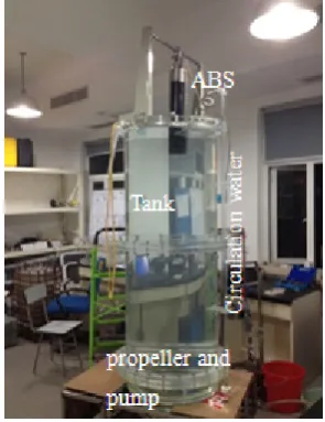
[image:2.595.357.505.469.661.2]The ABS was tested using FS (average particle size < 20 µm) and CS (average particle size > 100 µm). The experiments were conducted using the test tank system in the laboratory (Fig. 1). The system includes the test tank (600 mm diameter, 1500 mm height), the propeller and a pump at the bottom of the tank that recirculate the water, and a rubber tube to collect the water samples. The ABS (Aquatec Group Ltd, Hampshire, UK) equipped with sensors at acoustic frequencies of 0.5, 1, 2, and 4 MHz was mounted at the top of the tank facing directly down to the bottom of the tank. The FS and CS were obtained from sites in the Changjiang Estuary. The SSC in the test tank was relatively constant during each phase of the sampling. As the ABS was taking measurements, water samples were collected and analyzed separately for SSC and PS so that the ABS results could be compared with those determined using the traditional method (TM) [17]and the laser method (LM; i.e., using a laser diffraction particle size analyzer (Beckman Coulter, Miami, USA)).
Figure 1. The test tank used for the experiments
water samples for SSC and PS. The SSC values of the water samples were obtained using the TM, and the PS values were determined using the LM. The measured results were then compared with the SSC and PS results from the ABS backscatter strength data calculated using explicit (EASC) and implicit (IAMC, IASC, and IAMP) models (Appendix A).
4. Results
Figure 2 shows the SSC results from the water samples determined using the TM. The SSC values of FS varied from 0.18 to 0.34 g l–1 (Fig. 2a), and the SSC values of CS varied
from 0.18 to 0.68 g l–1 (Fig. 2b). Peak value of SSC was
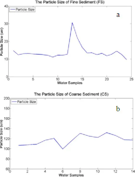
[image:3.595.318.548.80.380.2]found in the FS samples (Fig. 2a). Figure 3 shows the mean PS values of FS and CS in the water samples determined using the LM. The PS of FS varied from 9.7 to 30.6 µm, and the average value was 14 µm (Fig. 3a). The value for CS varied from 99.4 to 131.9 µm, with an average value of 118 µm (Fig. 3b).
Figure 2. Suspended sediment concentration (SSC) of (a) fine and (b)
coarse sediment in the water samples
Figure 3. Mean particles size (PS) of (a) fine and (b) coarse sediment in
the water samples
[image:3.595.64.292.330.642.2]Figure 4. Suspended sediment concentration (SSC) of (a-c) fine sediment (FS) and (d-f) coarse sediment (CS) obtained by the ABS and Traditional Method(TM)
Figure 5. Particle size (PS) of (a) fine sediment (FS) and (b) coarse sediment (CS) measured by the ABS and the laser method (LM)
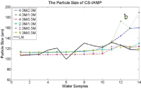
Tables 1 and 2 show the relationship (R2) between SSC/PS
obtained from the water sample measurements and the ABS results for FS and CS, respectively. The values of SSC calculated using the EASC, IASC, and IAMC models are from the 2 MHz sensor, and that of PS calculated using the IAMP model is from the ratio of the form functions of two frequencies (2/1 MHz). For SSC, the R2 value for the EASC
[image:5.595.53.302.435.523.2]model (explicit approach) was usually lower than those of the IASC and IAMC models (implicit approaches), and the value for EASC for CS was higher than that for FS. For PS, the R2 value for CS was higher than that for FS.
Table 1. The linear relative coefficient (R2) between suspended sediment
concentration/particle size (SSC/PS) obtained from the water sample measurements and ABS results for fine sediment (FS)
FS Number of water samples
24 20 18 16 14 10
EASC 0.02 0.10 0.13 0.17 0.26 0.52
IASC 0.16 0.42 0.59 0.74 0.94 0.99
IAMC 0.04 0.22 0.48 0.62 0.86 0.92
IAMP 0.07 0.20 0.27 0.35 0.50 0.65
The values of SSC (EASC, IASC, IAMC ) are from the sensor at 2 MHz, and the value of PS
[image:5.595.53.301.603.691.2](IAMP) is from the ratio of the form functions of two frequencies (2MHz/1MHz).
Table 2. The linear relative coefficient (R2) between suspended sediment
concentration/particle size (SSC/PS) obtained from the water sample measurements and ABS results for coarse sediment(CS)
CS Number of water samples
14 13 12 11 10 9
EASC 0.39 0.49 0.57 0.64 0.71 0.75
IASC 0.06 0.47 0.83 0.84 0.88 0.90
IAMC 0.29 0.54 0.66 0.75 0.82 0.89
IAMP 0.36 0.46 0.52 0.58 0.69 0.79
The values of SSC (EASC, IASC, IAMC) are from the sensor at 2 MHz, and the value of PS
(IAMP) is from the ratio of the form functions of two frequencies (2MHz/1MHz).
5. Discussion
In this experiment, different models were used to calculate SSC and PS results from the ABS backscatter strength data. The explicit approach (EASC model) applied to both FS and CS (Fig. 4a,d) yielded better SSC results than those of implicit approach models IAMC and IASC (Fig. 4b,c,e,f). The advantage of the EASC method is that there is no need to know the system calibration parameter
k
t. Once the value of M is obtained,k
tcan be circumvented. If the PS in the water column varies, however, some a priori reference information is required, such as,β
r,M
r ,k
s, andξ
. The explicit approach is only applicable to a single frequency and it uses the assumption thata
s is constant in the water column above the seabed [5]. Actually, experiments in the lab and field have shown thata
s varies within a certain range.The implicit IASC and IAMC models provided information about SSC and the IMAP model provided data for PS in the water column. The fluctuations of SSC were smaller for FS than for CS when the IAMC and IASC models were used. This means that when used in a fine sediment environment, the ABS yielded reasonable results (Fig. 4b,c,e,f). Nevertheless, Tables 1 and 2 show that careful choice of frequencies and data analysis and processing methods are crucial to obtaining the best results. Unlike the explicit approach, the implicit approaches require the system calibration parameter (
k
t) and accuratea
sand M values, and a strict choice of frequencies and data analysis methods must be used [5].The results presented in Tables 1 and 2 show a linear relationship between the time-averaged ABS backscatter strength and the square root of SSC. Similar results were reported by other researchers [11,18,19,20,21]. The implicit approaches yielded higher R2 values (> 0.89 for 10 CS
samples and > 0.92 for 10 FS samples) than the explicit approach (0.79 for 10 CS samples and 0.65 for 10 FS samples). Nevertheless, the fluctuation of SSC in the ABS results obtained using the explicit approach (Fig. 4a,d) was smaller than that of the implicit approaches (Fig. 4b,c,d,e) to This result means that the implicit approaches might be more sensitive to changes of SSC [2, 22] than the explicit approach, but this premise requires further research. A new statistical method [12] recently was introduced for converting ABS backscatter strength data to SSC and PS values, and it yielded better results for CS (255 - 400 µm). This data processing method was not used in the present study.
The peak values (0.34 g l–1 SSC, 30.6 µm PS) occurred for
used, the ratio of the form functions of 2/1 MHz yielded the best result in this experiment (Fig. 5a,b). Thus, the particle radii derived from the 1 to 2 MHz backscatter information profiles may be suitable for the Changjiang Estuary and other environments [19, 23]. However, the results should be further researched using different types of sediment in different environments.
6. Conclusions
The development of acoustic technology to non-intrusively measure SSC and PS in the boundary layer with both high temporal and spatial resolution is of interest to many researchers. In the present study, SSC and PS were measured using an ABS equipped with sensors at four frequencies (0.5, 1, 2, 4 MHz). The measurements were conducted in the test tank in the laboratory. A linear relationship between the time-averaged ABS backscatter strength data and the square root of SSC was detected. The values of SSC obtained using model EASC were better than those obtained using models IAMC and IASC. The implicit approaches were much more sensitive to changes of SSC, thus these models require a strict choice of frequencies and data analysis methods. The results of the present study show that acoustic systems (such as ABS) using 1 to 2 MHz backscatter information profiles should be obtain reasonable results in the Changjiang Estuary. Thus, acoustic technology potentially could be used to monitor the SSC and PS profiles in estuarine and coastal environments, including FS environments. Furthermore, use of parallel measurements from instruments such as Optical Backscatter Sensors and Laser In-Situ Scattering and Transmissometry devices, in the field would increase the accuracy and reliability of ABS calibration and subsequent SSC and PS results.
Acknowledgements
This work was supported by the Technology of Development and Research Foundation of SKLEC (No.2013JSKF02), the Key Program of the National Natural Science Foundation of China (No. 41130856) and China Scholarship Council (No.201206145012). The authors are grateful to R. M. Wu, Q. Q. Bi, R.S. Wang, and Y. Shi for contributions to this experiment. The authors are also grateful to anonymous reviewers for their constructive suggestions and comments.
Appendix
1. Explicit Approach
Explicit Approach Sediment Concentration (EASC): if M and
k
sare known at the reference ranger
r, the following expression can be deduced:2 2 2
4
r r r r rM
dr
M
β
β
β ξ
=
−
∫
(3)
where
β
=
V r k e
rmsψ
s−1 2αr andβ
r=
β
atr r
=
r2. Implicit Approach
(1) Implicit Approach Single Frequency Concentration (IASC)
Rearranging Eq. (1)
Assuming the system has been calibrated: 2
4r w
rms s t
V
r
M
e
K K
αψ
=
(4)(2) Implicit Approach Multiple Frequency Concentration (IAMC)
If using multiple frequencies,
M
i can be obtained from: 24 2 2 r i
rmsi
i i
si ti
V
M
r e
K K
α
ψ
=
(5)where
i
refers to the different frequencies.(3) Implicit Approach Multiple Frequency Particle Size (IAMP)
Particle size can be obtained using the ratio of one frequency’s form function (
f
) to that of another frequency. If multiple frequencies are available,a
s need not be assumed and can be obtained.2 ( i j)
i avergei
r ti
i
j j avergej
tj
V
k
f
e
f
V
k
α αψ
ψ
−
=
(6)where
i j
≠
andi
andj
refer to the different frequencies (0.5, 1, 2, and 4 MHz in this study) [5,24].REFERENCES
[1] Thorne P. D. and Hurther D., 2014. An overview on the use of backscatter sound for measuring suspended particle size and concentration profiles in non-cohesive inorganic sediment transport studies. Continental Shelf Research, 73, 97-118. [2] Thorne P. D., Hurther D., Moate B. D., 2011. Acoustic
[3] Rai A. K. and Kumar A., 2015. Continuous measurement of suspended sediment concentration: Technological advancement and future outlook. Measurement, 76, 209 -227. [4] Holdaway G. P.,Thorne P. D., Flatt D., Jones S. E., Prandle D., 1999. Comparison between ADCP and transmissometer measurements of suspended sediment concentration. Continental Shelf Research, 19, 421-441.
[5] Thorne P. D., Hanes D. M., 2002. A review of acoustic measurement of small-scale sediment process. Continental Shelf Research, 22, 603-632.
[6] Guerrero M., Szupiany R.N., Amsler M., 2011. Comparison of acoustic backscattering techniques for suspended sediments investigation. Flow Measurement and instrumentation, 22, 292-401.
[7] Guerrero M, Szupiany R., Latosinski F., 2013. Multi-frequency acoustics for suspended sediment studies: an application in the Parana River. Journal of Hydraulic Research, Vol. 51, No. 6, 696-707.
[8] Hay A. E., Sheng J., 1992. Vertical profiles of suspended sand concentration and size from multifrequency acoustic backscatter. Journal of Geophysical Research, 97(C10):156, 61-77.
[9] Betteridge K. F. E., Thorne P. D., Cooke R D., 2008. Calibrating multi-frequency acoustic backscatter systems for studying near-bed suspended sediment transport processes. Continental Shelf Research, 28, 227-235.
[10]Moate B. D., Thorne P. D., 2012. Interpreting acoustic backscatter from suspended sediments of different and mixed mineralogical composition. Continental Shelf Research, 46, 67-82.
[11]Hunter T. N., Darlison L, Peakal J l, Biggs S, 2012. Using a multi-frequency acoustic backscatter system as an in situ high concentration dispersion monitor. Minerals Engineering, 27-28, 20-27.
[12]Wilson G.W. and Hay A.E., 2015. Acoustic backscatter inversion for suspended sediment concentration and size: A new approach using statistical inverse theory. Continental Shelf Research, 106, 130 -139.
[13]MacDonald I. T., Vincent C. E., Thorne P. D., and Moate B. D., 2013. Acoustic scattering from a suspension of flocculated sediments. Journal of Geophysical Research: Oceans, 118, 2581-2594, doi:10.1002/jgrc.20197.
[14]Bux J., Peakall J., Biggs S., Hunter T. N., 2015. In situ characterisation of a concentrated colloidal titanium dioxide
settling suspension and associated bed development: Application of an acoustic backscatter system. Powder Technology, 284, 530 -540.
[15]Hay, A.E., 1991. Sound scattering from a particle-laden turbulent jet. Journal of the Acoustical Society of America, 90, 2055-2074.
[16]Thorne, P. D., Hardcastle P. J., Dolby J. W., 1998. Investigation into the application of cross-correlation analysis on acoustic backscattered signals from suspended sediment to measure nearbed current profile. Continental Shelf Research, 18(6), 695-714.
[17]Zhang W. X., Yang S.L, Zhu J., Gong S.L., Ding P.X., 2007. Dry season variability in suspended sediment concentration in the south passage of the Changjiang Estuary. International Journal of Sediment Research. Vol. 22, No.3, 199-207. [18]Hay A. E., 1983. On the Remote Acoustic Detection of
Suspended Sediment at Long Wavelengths. Journal of Geophysical Research, 1983, Vol. 88, No. C12, 7525-7542. [19]Thorne, P. D. and Hardcastle P. J., 1997. Acoustic
measurements of suspended sediments in turbulent currents and comparison with in-situ samples. Journal of the Acoustical Society of America, 101(5, Part 1): 2603-2614. [20]Hoitink A.J.F. and Hoekstra P., 2005. Observations of
suspended sediment from ADCP and OBS measurements in a mud-dominated environment. Coastal Engineering, 52,103-118.
[21]Guerrero M., Rüther N., Szupiany R.N., 2012. Laboratory validation of acoustic Doppler current profiler (ADCP) techniques for suspended sediment investigations. Flow Measurement and Instrumentation, 23, 40-48.
[22]Holdaway, G. P. and Thorne, P. D., 1997. Determination of a fast and stable algorithm to evaluate suspended sediment parameters from high resolution acoustic backscatter systems. Seventh International Conference on Electronic Engineering in Oceanography, Southampton Oceanography Centre, UK, 23-25 June, 86-92.
[23]Hurther D., Thorne P. D., Bricault M, Lemmin U, Barnoud J. M., 2011. A multi-frequency Acoustic Concentration and Velocity Profiler (ACVP) for boundary layer measurements of fine-scale flow and sediment transport processes. Coastal Engineering, 58, 594-605.