Cointegration between Government Expenditure and Revenue: Evidence from India

Cointegration between Government Expenditure and

Revenue: Evidence from India

Asit Ranjan Mohanty

_{, Bibhuti Ranjan Mishra}

1_{Faculty of Accounting and Finance, Xavier Institute of Management, Xavier University, India}

2_{Centre of Excellence in Fiscal Policy and Taxation (CEFT), Xavier Institute of Management, Xavier University, India}

Copyright©2017 by authors, all rights reserved. Authors agree that this article remains permanently open access under the terms of the Creative Commons Attribution License 4.0 International License

Abstract

revenue of the government and public expenditure in India using Johensen-Juselius cointegration Methodology during 1980-81 to 2013-14. It tests four hypotheses relating to the revenue-expenditure nexus, i.e. tax-spend hypothesis, spend-tax hypothesis, fiscal synchronization hypothesis and institutional separation hypothesis. The nexus is studied at centre, state and combined level. The study establishes one cointegrating relationship between public expenditure and tax revenue which suggests a long-run relationship between the two. The results of the Vector Error Correction Models evince that there is one-way causality running from tax revenue to expenditure both in short-run as well as in the long-run. This result justifies the operation of tax-spend hypothesis. The reverse-causality is not found in the analysis either for short or long-run.

Keywords

Cointegration, Vector Error Correction Models, Granger Causality Test

1. Introduction

The adverse macroeconomic impact of budget deficits on national saving and investment, and thereby the potential growth of a nation has drawn considerable attention by many researchers and policy makers. In assessing the role of the government in redistribution of resources, it is essential to understand the relationship between government expenditure and revenue. In case of India, Fiscal Policy was also given importance to achieve growth and equity with social justice. The government indulges in taxation and expenditure policies to redistribute the income and wealth for the betterment of the poor and needy. By and large, the central as well as the state government accrue surpluses in their revenue account during the first three decades since the time India got independence [1]. But, during the 1980s and 1990s, the condition of major fiscal indicators has worsened

implying the issue of growing resource gap over time. The growing revenue deficit and fiscal deficit during 1980 to 2002 compelled the Government of India to enact the Fiscal Responsibility and Budget Management (FRBM) Act in 2003 wherein fiscal targets were earmarked with provisions to boost revenue and cut-down unproductive expenditure.1

The State governments also enacted the FRMB Act in their respective states in different years. Karnataka is the first state to enact the FRBM Act in September 2002, while West Bengal is the last state in implementing the Act in July 2010. After 2003, the deficit indicators showed an improvement which lasted till 2007-08, the eventful year of global crisis. After the global economic crisis, the condition of these indicators again deteriorated with the exception of states. In recent years, the rapid increase in fiscal deficit and revenue deficit in India mainly contributed by the central government has generated renewed interest on the topic.

Table 1. Deficit Scenario in Centre and State (as % of GDP) Indicator Revenue Deficit Gross Fiscal Deficit

Year Centre State Combined Centre State Combined 1980-89 1.67 -0.08 1.56 6.56 2.76 7.72 1990-99 2.94 1.17 4.07 5.72 3.00 7.49 2000-02 4.15 2.46 6.54 5.74 4.00 9.38 2003-2007 2.26 0.44 2.67 3.61 2.67 6.22 2008-2013 4.19 -0.05 4.14 5.56 2.24 7.77 Note: Negative values indicate surplus. Data collected from Handbook of Statistics in Indian Economy, RBI.

To answer the question on how to correct the deficit situation, the nexus between government revenue and expenditure plays an important role. To a major extent, the relationship between the two depends on how the deficits are financed. Deficit can be financed through printing new money, domestic borrowing or foreign borrowing. If the deficit is financed through seigniorage or printing new money, then it will create inflation situation with increased

government spending which could initiate a debt spiral and consequently a higher expectation in taxes. Domestic borrowing is perceived as a way to avoid both inflation and external crises, but it has its own limitations if used excessively. Excessive external borrowing could result in external crisis or crisis in balance of payments front. In India deficit is mainly financed through public borrowings which can lead to more taxation in future. There are several competing studies examining the relationship between government revenue and government expenditure. A detailed review of roughly 56 studies on the tax-spend debate is provided by Payne [2]. It can be observed from the literature that the results are time specific, country specific, methodology used etc.

The inconclusive results of earlier studies and limited studies in case of India, provides an impetus to examine the government’s revenue-expenditure nexus. The study employs the Johensen-Juselius Maximum likelihood approach to explore the cointegration relation between the two followed by the vector error correction models (VECM). In short the study validates the tax-spend hypothesis. The remainder of this study is structured as follows: the second section gives the theoretical background of the study. Third Section provides a survey of contemporary literature. The Fourth section outlines the objective and data used in the study. The Fifth section provides the empirical model and methodology. The Sixth section outlines the empirical results. Seventh Section delineates concluding observations and some policy implications.

2. Theoretical Background

The co-integration between revenue and expenditure is based upon the premise that revenue impacts expenditure of the government. This implies that the government does not want either high revenue deficit or fiscal deficit to finance expenditure. In other words, the expenditure is limited by revenue receipts. On the other hand, government expenditures may affect its revenue which is the opposite of the first one. Here, it is implicit that expenditures of the government lead to change the tax rate and non-tax structure in order to finance expenditure. It may also happen that both revenue and expenditure decisions will be undertaken simultaneously. In this case, there is no relationship could be established between revenue and expenditure.

Indian economy faced with the problem of large fiscal deficit and the monetization of budget deficit adversely affected external sector in the late 1980s and early 1990s. The large borrowings of the government led to debt un-sustainability situation and the paying capacity of the government was not enough to pay even for two weeks of imports. This had led to economic crisis of 1991. Consequently, structural reforms were introduced in 1991 and fiscal sustainability through fiscal consolidation emerged as one of the key areas of economic reforms. To contain rising fiscal deficit, the Government introduced

FRBM Act, 2003 to check the deteriorating fiscal situation. Fiscal Responsibility and Budget Management (FRBM) Act was introduced in 2003 in order to ensure prudent fiscal management, macroeconomic stability, coordination between fiscal and monetary policy, and transparency in fiscal situation of the Government. The FRBM Act is a set of fiscal rule that specifies a cap on fiscal deficit at 3% of the GDP (GSDP for States) with zero revenue deficit. It has also put a ceiling on both debt and interest payment ratio. The entire objective is to contain expenditure of both Union and State Government to operate within their means. FRBM Act provides a legal institutional framework for fiscal consolidation. It is now mandatory for both the Central and State governments to take measures to reduce fiscal deficit, eliminate revenue deficit and generate revenue surplus in the subsequent years.

In this theoretical backdrop, it is quite important to empirically examine the relationship between revenue and expenditure as well as their direction of causality in both long run and in short run both at the Centre and State Government level.

3. Review of Literature

On the nexus between government revenue and government expenditure, four main hypotheses could be inferred from literature. First one is the ‘Tax-Spend’ hypothesis which sees a causal flow running from revenue to expenditure. One of the proponents of this hypothesis was Friedman [3] who claims that increase in taxes will result in increase in expenditure and reduction of budget deficit will be a distance dream. Subsequently, Buchanon and Wagner [4] approve the impact of revenue and expenditure with different explanation by bifurcating direct and indirect taxation. According to them indirect taxation leads to more government spending. If the public spending is financed by other means of taxation than the direct tax, then the public observes the price of government spending to be more with direct taxation than that under indirect taxation. The indirect taxation begins through higher interest rates as a result of higher spending and inflation due to crowding out effect. Hence, the framework of Buchanan-Wagner provided a ground where a higher tax will lead to a decrease in government spending in the presence of fiscal illusion which is the opposite of Friedman’s contention. In econometric terminology, this hypothesis implies a unidirectional causality running from revenue to expenditure.

Taking cue from the Ricardian equivalence, Barro [7, 8] contends that today’s public borrowing will culminate in increasing the future tax liability of the people. Hence, he rejected the presence of fiscal illusion wherein increase in government spending leads to increase in taxes. In an empirical sense this hypothesis postulates a unidirectional causality running from expenditure to revenue.

The third hypothesis is known as ‘Fiscal Synchronization’ hypothesis, wherein revenue and expenditure decisions are taken simultaneously as voters of a country usually compare the marginal benefits and costs of government services simultaneously (Musgrave [9], Meltzer and Richard [10]). In an empirical sense this implies a bi-directional causality between expenditure and revenue.

The fourth one could be termed as ‘Institutional Separation’ or Neutrality Hypothesis wherein no relationship could be established between revenue and expenditure. Wildavsky [11], Hoover and Sheffrin [12] and Baghestani& McNown [13] argued that as there is institutional separation in taking government spending and revenue decisions, there could be no inherent relationship between the two. Econometrically, this hypothesis suggests no causality between revenue and expenditure.

The empirical work on the tax-spend debate has shown mixed results due to the time periods analysed, field of study, methodology used etc. Usually, many studies used Granger causality test either in a vector autoregressive framework or within an error correction system.

Some studies find support for tax-spend hypothesis [12, 14-18], while the reverse-causality or spend-tax hypothesis is validated by others [19-24]. Some papers support the fiscal synchronization hypothesis [25-28], while Baghestani and McNown [13] support the institutional separation hypothesis. Owoye [29] while examining the tax-spend hypothesis in G-7 countries, get evidence of fiscal synchronization hypothesis for all the countries except Japan and Italy. For these two countries tax-spend hypothesis holds well.

Ram [30] explores the spend-tax debate by taking 22 countries comprising of developed and less developed countries. He gets support for the tax-spend hypothesis in Philippines, El Salvador, Thailand, and the United Kingdom.Spend-tax hypothesis was validated in case of Honduras and New Zealand.Fiscal synchronization was suggested in only one country that is Nicaragua. Rest of the eighteen countries show evidence of institutional separation hypothesis. Joulfaian and Mookerjee [31] examined the OECD countries and get support of tax-spend hypothesis in Italy and Canada. Spend-tax hypothesis is validated for the Japan, France, United States, Germany, United Kingdom, Austria, Finland, and Greece. Fiscal synchronization hypothesis is supported only in case of in Ireland. Baffes and Shah [32, 33] have prolonged this analysis for Argentina, Brazil, Chile, Mexico, and Pakistan. They find support of fiscal synchronization hypothesis for Brazil, Mexico, and Pakistan while for Argentina and Chile spend-tax hypothesis is supported. Ewing and Payne [34] examine the revenue and expenditure relationship for Latin American countries. They

find support of fiscal synchronization hypothesis for Chile and Paraguay; support for tax-spend hypothesis in case of Colombia, Ecuador, and Guatemala. Paleologou [35] explored the relationship of revenue and expenditure in three countries using a non-linear framework with structural break. The study finds support for synchronization hypothesis for Sweden and Germany and validated the spend-tax hypothesis for Greece. Few other studies examined the revenue-expenditure nexus in non-linear framework [36-39]. Recent studies also extended the analysis to subnational and local governments [40-45].

In case of India, Bhat et al. [46], using state level data find the evidence of fiscal synchronization hypothesis. Das and Das [47] using cointegration and Granger causality got bidirectional causality between nominal revenue and nominal expenditure. But they got support of spend-tax hypothesis when real values of the data were taken for the centre. Dhanasekaran [48] got mixed result using two methodologies. Spend-tax hypothesis is validated with Granger Causality, while fiscal synchronization is validated partially with Gweke decomposition method. Naidu et al. [49], using Granger and Sim-test of causality get support of fiscal synchronization hypothesis in case of the state of Andhra Pradesh, India. A recent study by Bishnoi and Teja [50] shows the evidence of tax-spend hypothesis in case of the state of Haryana, India.

4. Objective and Data

Table 2. Descriptive Statistics of Natural log of Various Variables Variables CAE CTR SAE STR AE TR

Mean 7.65 7.14 7.63 6.56 8.33 7.59 Median 7.68 7.20 7.66 6.58 8.36 7.63 Maximum 9.65 9.42 9.83 8.94 10.44 9.90 Minimum 5.43 4.88 5.42 4.19 6.12 5.29 Std. Dev. 1.24 1.32 1.31 1.37 1.27 1.34 Skewness -0.09 0.02 -0.05 0.00 -0.07 0.02 Kurtosis 1.95 1.93 1.86 1.92 1.90 1.92 Note: AE and TR denote Aggregate Expenditure and Tax Revenue of combined Centre and State. Prefix C and S denote the respective variables for the Centre and State, correspondingly.

consists of Direct and Indirect Taxes. In the State level State own tax revenue is considered which is net of shared tax. Total expenditure is constituted of revenue and capital expenditure. The descriptive statistics of the variables used in the analysis are given in Table-2.

5. Econometric Methodology

This paper applies the Johansen [51, 52] cointegration procedure to test the existence of a long run relationship between public expenditure and revenue.2 _{Following two}

models are fitted to examine the tax-spend and spend-tax hypotheses.

𝐴𝐴𝐴𝐴𝑡𝑡= 𝑎𝑎0+ 𝑎𝑎1𝑇𝑇𝑇𝑇𝑡𝑡+ 𝑒𝑒1𝑡𝑡 (1) 𝑇𝑇𝑇𝑇𝑡𝑡= 𝑏𝑏0+ 𝑏𝑏1𝐴𝐴𝐴𝐴𝑡𝑡+ 𝑒𝑒2𝑡𝑡 (2) Where, AE is Aggregate Expenditure, TR is Tax Revenue, 𝑎𝑎0 and 𝑏𝑏0 are intercepts, 𝑎𝑎1 and 𝑏𝑏1 are coefficients, and 𝑒𝑒1𝑡𝑡 and 𝑒𝑒2𝑡𝑡 are the associated error terms.

5.1. Unit Root Test

To avoid spurious regression situation, the variables must be stationary or cointegrated. So, the first step in the procedure is to determine the stationarity and the order of integration of each time series. A time series is integrated of order 1, that is, I(1) if it becomes stationarity after it is differenced once. We use the Phillips–Perron (PP) [54, 55] procedures to test the stationarity of different variables. The PP Test distinguishes itself from ADF test in how they deal with serial correlation and heteroskedasticity in errors. While the ADF test uses a parametric auto-regression to approximate the ARMA structure of the errors in the test regression, the PP test ignores any serial correlation in the test regression. The test regression for PP test is as follows.

∆𝑦𝑦𝑡𝑡= 𝛽𝛽′𝐷𝐷𝑡𝑡+ 𝜂𝜂𝑦𝑦𝑡𝑡−1+ 𝓊𝓊𝑡𝑡 (3) Where, 𝓊𝓊𝑡𝑡 is I (0) and can be heteroskedastic. The serial correlation and heteroskedasticity in errors (𝓊𝓊𝑡𝑡) is corrected in PP test by directly modifying the test statistics, 𝑡𝑡𝜂𝜂=0 and 𝑇𝑇𝜂𝜂̂. Under the null hypothesis that is 𝜂𝜂 = 0, the PP test follows a Z-distribution and the estimated statistics have the same asymptotic distributions as the ADF t-statistic and normalized bias statistics. PP test has two advantages over ADF statistics that are 1. The PP tests are robust to general forms of heteroskedasticity in the error term 𝓊𝓊𝑡𝑡, and 2. No need to specify a lag length instead the Newey-west bandwidth is given to accommodate for structural change.

5.2. Johansen-Juselius Cointegration Test

If two series are I (1) but their linear combination is

2 For bivariate model, Engle–Granger [53], 2-step procedure of cointegration was also used in the literature. But we rely on Johensen-Juseleous Maximum likelihood estimator as it is improved than the former.

stationary, the series are said to be cointegrated. To test for cointegration, we will use the Johensen-Juselius (JJ) method that is based on the maximum likelihood estimation procedure. If cointegration exists, the number of cointegrating vectors would be determined. The JJ procedure for our proposed model is a vector auto-regressive (VAR) model which can be estimated in order to examine the cointegration relationship. To begin with we admit Zt as the

(2 × 1) vector consisting of aggregate expenditure (AE) and Tax Revenue (TR).3 _{Thus, the autoregressive model of Z}

t

can be expressed as follows.

𝑍𝑍𝑡𝑡= 𝜇𝜇 + 𝛿𝛿1 𝑍𝑍𝑡𝑡−1+ 𝛿𝛿2 𝑍𝑍𝑡𝑡−2+ … … … . +𝛿𝛿𝑘𝑘𝑍𝑍𝑡𝑡−𝑘𝑘+ 𝜀𝜀𝑡𝑡 (4) The long-run equilibrium for Equation (4) is when 𝛿𝛿𝛿𝛿 = 0.

Where, 𝛿𝛿 is a (2 × 2) coefficient matrix(1 − 𝛿𝛿1− 𝛿𝛿2− … … . . −𝛿𝛿𝑘𝑘). The rank of (r ≤ 2) of 𝛿𝛿 determines the number of cointegrating vectors. If the variables are cointegrated, the cointegrating rank is given as 𝛿𝛿 = 𝛼𝛼𝛽𝛽′_{, where α is the} matrix of parameters denoting the speed of convergence to the long-run equilibrium and β represent the (2 × r) matrices of parameters of the cointegrating vector. The rows of (𝛽𝛽′₎ form the r cointegrating vectors such that if (𝛽𝛽′

𝑗𝑗) is the ( jth) row of 𝛽𝛽′_{, 𝛽𝛽}′

𝑗𝑗𝑍𝑍𝑡𝑡 ~ 𝐼𝐼(0).

In succession, JJ derived two likelihood ratio test statistics for testing the number of cointegrating rank in the system which are trace test (𝜆𝜆𝑡𝑡𝑡𝑡𝑡𝑡𝑡𝑡𝑡𝑡) and maximum Eigen values test(𝜆𝜆𝑚𝑚𝑡𝑡𝑚𝑚.) as can be shown in Equation (5) and (6) respectively.

𝜆𝜆𝑡𝑡𝑡𝑡𝑡𝑡𝑡𝑡𝑡𝑡= −𝑇𝑇 ∑𝑛𝑛𝑖𝑖=𝑡𝑡+1ln(1 − 𝜆𝜆𝑖𝑖) (5) 𝜆𝜆𝑚𝑚𝑡𝑡𝑚𝑚= −𝑇𝑇 ln (1 − 𝜆𝜆𝑡𝑡+1) (6) Where 𝜆𝜆, is the estimated Eigen values and T is the number of observations. If the test statistic is greater than the critical value, this indicates the rejection of hypothesis of full rank or the null hypothesis of no cointegration relationship.

5.3. VECM Model

Once it is established that there is cointegration among the three variables, there must exist some Granger causality [56]. Hence, we can use Granger-causality test to examine the nature of the relationship among them. According to Engle and Granger [53], if the variables are cointegrated, Granger causality test within the first difference VAR model will be misleading. Therefore, an error-correction term should be included into the model to capture the equilibrium relationship among the cointegrating variables in their dynamic behaviour. Two vector error correction models (VECM) can be formulated for the two models as follows.

∆𝐴𝐴𝐴𝐴𝑡𝑡= 𝛼𝛼10+ ∑𝑖𝑖=1𝑘𝑘 𝜗𝜗11∆ 𝐴𝐴𝐴𝐴𝑡𝑡−𝑖𝑖+ ∑𝑘𝑘𝑖𝑖=1𝜗𝜗12∆ 𝑇𝑇𝑇𝑇𝑡𝑡−𝑖𝑖+ 𝜑𝜑1𝐴𝐴𝐸𝐸𝑡𝑡−1+ 𝜀𝜀1𝑡𝑡(7)

3 For Centre and States, expenditure is represented by CAE and SAE, respectively. Tax variable for Centre and States is denoted as CTR and STR respectively.

∆𝑇𝑇𝑇𝑇𝑡𝑡= 𝛼𝛼20+ ∑𝑖𝑖=1𝑘𝑘 𝜗𝜗21∆ 𝑇𝑇𝑇𝑇𝑡𝑡−𝑖𝑖+ ∑𝑘𝑘𝑖𝑖=1𝜗𝜗22∆ 𝐴𝐴𝐴𝐴𝑡𝑡−𝑖𝑖+ 𝜑𝜑2𝐴𝐴𝐸𝐸𝑡𝑡−1+ 𝜀𝜀2𝑡𝑡(8) Where, ∆ is the first difference operator and the residuals 𝜀𝜀𝑖𝑖𝑡𝑡 (i = 1, 2) are assumed to be normally distributed and white noise. From the above equations, 𝐴𝐴𝐸𝐸𝑡𝑡−1 is the one period lagged error-correction term derived from the cointegrating equation. The coefficient of the 𝐴𝐴𝐸𝐸𝑡𝑡−1 term infers the long run causality, while the joint F-test of the coefficients of the first differenced explanatory variables depict the short run causality. For short period, the causality can be derived through the Wald test of the joint significance of the lags of the independent variables. The joint test of lagged variables, that is, ∆𝐴𝐴𝐴𝐴𝑡𝑡 and ∆𝑇𝑇𝑇𝑇𝑡𝑡 by mean of the F-statistic is significantly different from zero, implies the presence of Granger causality. For example, if the joint test of lagged variables of ∆𝑇𝑇𝑇𝑇𝑡𝑡 in equation (7) is significantly different from zero, then it implies that tax revenue growth Granger causes expenditure growth. We took the optimal lag length of 3 in the VECM system by considering the Akaike Information Criterion (AIC) statistic. In addition to this we have done several diagnostic tests like Jarque-Bera test for normality, Ramsey’s RESET test for functional misspecification and Breusch-Godfrey LM test for serial correlation.

6. Empirical Results

6.1. Unit Root Test

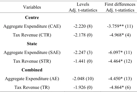
The unit root test is performed using the Phillips & Perron procedure on both the level and first difference of the variables. This test suggests that the variables are non-stationary at level and stationary at the first difference (Table-3). From this test it can be inferred that there could be existence of long run relationship between government tax revenue and government expenditure. In the Unit root test the truncation lag is selected by following Newey-West Method using Barlett Kernel spectral estimation method.

Table 3. Phillips-Perron Unit Root Test (with trend and intercept) Variables _{Adj. t-statistics} Levels First differences _{Adj. t-statistics}

Centre

Aggregate Expenditure (CAE) -2.220 (8) -3.759** (11) Tax Revenue (CTR) -2.178 (0) -4.968* (4)

State

Aggregate Expenditure (SAE) -2.247 (3) -6.097* (11) Tax Revenue (STR) -1.441 (0) -4.464* (12)

Combined

Aggregate Expenditure (AE) -2.048 (10) -4.450* (13) Tax Revenue (TR) -1.926 (0) -4.864* (6)

Notes: Figure in parenthesis is Band-width selected by the Newey-West Method using Barlett Kernel. * and ** denote rejection of the null hypothesis of unit root at 1% and 5% level of significance. Adjusted t-statistics are as reported by MacKinnon (1996).

6.2. Cointegration Test

The results obtained from the unit root tests suggested that all the variables are integrated of order one. Therefore, we proceed to test long-run relationship between tax revenue and expenditure using Johansen & Juselius cointegration test. The optimal lag length of three is chosen by following the Akaike Information Criterion and considering the statistical significance. The test statistics are estimated with the assumption of no deterministic trend in the level data but presence of intercepts in the cointegrating equations. The test is done at three levels, i.e. Centre, State and combined. The results are presented in Tables 4. Results indicate that at the 5 percent level of significance, both the maximum eigenvalue and trace statistics suggest existence of one cointegrating vector between Tax Revenue and Expenditure at Centre, State and Combined Centre-State level.

The normalized cointegrated vector is estimated and depicted in Table-5 as follows. The results corroborate with our expectation that the long-run relationship between tax revenue and expenditure is positive. A 1% increase in tax revenue generates a 0.92%, 0.95% and 0.94% increase in expenditure in Centre, State and Combined level respectively. The significant impact of Tax revenue on expenditure validates the Tax-Spend hypothesis in case of India.

Table 4. Maximum Likelihood estimates of Number of Co-integrating Vectors

Null Alternative λmax λtrace Centre

𝑟𝑟 = 0 𝑟𝑟 = 1 16.3302** 16.5192**

𝑟𝑟 ≤ 1 𝑟𝑟 = 2 0.1889 0.1889

State

𝑟𝑟 = 0 𝑟𝑟 = 1 16.5465** 17.0595**

𝑟𝑟 ≤ 1 𝑟𝑟 = 2 0.5130 0.5129

Combined

𝑟𝑟 = 0 𝑟𝑟 = 1 21.0596** 21.0630**

𝑟𝑟 ≤ 1 𝑟𝑟 = 2 0.0034 0.0034

Notes: ** Denotes rejection of the Null Hypothesis of no co-integration at the 0.05 level. Critical values are as reported by MacKinnon-Haug-Michleis (1999).

While estimating receipts and expenditure for allocation of resources to different sector in the Budget (Annual Financial Statement) of particular financial year, the government first makes a projection of growth in output.4

Subsequently, from historical data, the elasticity of revenue receipts (both tax & non tax revenue) is estimated to find out expected revenue receipts. This is followed resource expected mobilization through capital receipts which include both of debt receipts and non-debt receipts. The mobilization of debt receipts is budgeted based upon the debt sustainability of the government. The budgeted receipts are used to finance expenditure in general services, social

4 Centre and State Government project GDP and GSDP respectively.

services and economic services sector by way of both revenue and capital expenditure. While financing expenditure, the priorities of the government are taken into consideration. Expenditures in different sectors of the economy generate output growth through multiplier effect. This process continues in each budget. If there are any deviation receipts / expenditure or both, government revises the budget estimate. Hence, co-integration between revenue and expenditure is established through output growth. Our empirical results established the co-integration between revenue and expenditure through one common vector i.e. output growth.

Table 5. Long-run Relationship among Revenue and Expenditure Level Normalized Co-integrating Vector Centre CAE=1.1183+0.9164 CTR

(0.0108) State SAE=1.3858+0.9527 STR

(0.0058) Combined AE=1.2207+0.9388 TR

(0.0071) Note: Standard Error in Parenthesis

6.3. VECM Models

Table 6. Granger Causality between Revenue and Expenditure

Centre

Dependent Δ CAE ΔCTR ECT (-1) P-value Δ CAE --- 3.0723*** -0.4944 0.0009 ΔCTR 0.2341 --- -0.0291 0.2549

State

Dependent ΔSAE ΔSTR ECT (-1) P-value ΔSAE --- 2.5070*** -0.9096 0.0006 ΔSTR 0.2916 ---- 0.1403 0.5145

Combined

Dependent ΔAE ΔTR ECT (-1) P-value ΔAE --- 4.2808** -0.5890 0.0002 ΔTR 0.5581 ---- -0.2521 0.2896 Note: ** and ** Indicate F-values significant at 5% and 10% Level.

As we find one cointegrating vector while testing the long-run relationship between tax revenue expenditure, following the Granger Representation Theorem an error correction term can be added to each equation of the first differenced model to capture the equilibrium relationship between the variables in a dynamic set-up. In relation to the cointegration relationship, the vector error correction models are estimated which are exhibited in Table-6. In the expenditure equation, the error term is found to be negative and statistically significant irrespective of the level of study. It signifies a long run causality running from tax revenue to expenditure. The coefficient of error term shows the speed of adjustment wherein the system corrects its previous year’s disequilibrium. In the expenditure equation the error correction term is found to be -0.49, -0.91 and -0.58 in case of Centre, State and Combined level respectively. The

F-statistic of lagged coefficient of tax-revenue is found to be significant at 10% level for the centre and state, and significant at 5% level for the combined tax. It evinces a short-run causal flow running from tax revenue to expenditure. In the Tax revenue equation, the error term and the coefficient of lagged expenditure term are found to be insignificant which denies any possibility of long-run or short-run causality from expenditure to tax revenue.

We have also done several diagnostic tests like Jarque-Bera test for normality, Ramsey’s RESET test for functional misspecification and Breusch-Godfrey LM test for serial correlation (not reported here). The results of these tests do not violate these assumptions. Further, the error correction models are also dynamically stable as the characteristic roots are found to be within the unit circle.

7. Concluding Remarks and Policy

Implication

The study examines the nexus between tax revenue of the government and public expenditure in India using Johensen-Juselius co-integration Methodology. It tests four interrelated hypotheses relating to the revenue-expenditure nexus, i.e. tax-spend hypothesis, spend-tax hypothesis, fiscal synchronization hypothesis and institutional separation hypothesis. The nexus is studied for centre, state and combined level. The study establishes one co-integrating relationship between public expenditure and tax revenue which suggests a long-run relationship between the two. The results of the Vector Error Correction Models evince that there is one-way causality running from tax revenue to expenditure both in short-run as well as in the long-run. This result justifies the operation of tax-spend hypothesis in India. The reverse-causality is not found in the analysis either for the short-run or long-run.

As regards to the policy implication, the findings of this study will help both the state governments and central government in formulating their annual budget. Considering the results obtained from this study, the budget formulation of the governments should start with computation of earnings from tax and non-tax revenue by making appropriate projections of Gross Domestic Product and consumption pattern of the people. Depending upon the tax base and tax rate, the total revenue could be forecasted. Thereafter, resource allocation could be done effectively.

8. Highlights

 The study has identified long-run relationship between public expenditure and tax revenue.

 There is impact of the tax revenue on expenditure both in the short-run as well as in the long-run.  The reverse-causality is not found in the analysis

REFERENCES

S. M. Pillai, S. Chatterjee, B. Singh, S. Das, A. Gupta. Fiscal [1]

Policy: Issues and Perspective, Reserve Bank of India- Occasional papers, Vol. 18 (2 & 3), Special Issue, June & September, 1997.

J.E. Payne. A Survey of the International Empirical Evidence [2]

on the Tax-Spend Debate, Public Finance Review, Vol. 31, No. 3, 302-324, 2003.

M. Friedman. The limitations of tax limitation, Policy Review, [3]

Summer, 7–14, 1978.

J. Buchanan, R. Wagner, Democracy in Deficit, New York: [4]

Academic Press, 1977.

A. Peacock, J. Wiseman. Approaches to the Analysis of [5]

Government Expenditures Growth, Public Finance Quarterly, January, 3-23, 1979.

P. C. Roberts. Idealism in public choice theory. Journal of [6]

Monetary Economics (August), 603-16, 1978.

R.J. Barro. Are Government Bonds Net Wealth? Journal of [7]

Political Economy, November/December, 1095-1118, 1974. R.J. Barro. On the determination of public debt, Journal of [8]

Political Economy, Vol. 87, pp. 940-71, 1979.

R. Musgrave. Principles of Budget Determination, Public [9]

Finance: Selected Readings, eds. by H. Cameron and W. Henderson, New York: Random House, 1966.

A. Meltzer, S. Richard. A Rational Theory of the Size of [10]

Government, Journal of Political Economy, Vol. 89, 914-927, 1981.

A. Wildavsky. The new politics of the budgetary process. [11]

Glenview, IL: Scott, Foresman, 1988.

K.D. Hoover, S.M. Sheffrin. Causation, Spending, and Taxes: [12]

Sand in the Sandbox or the Tax Collector for the Welfare State? American Economic Review, Vol. 82 (1), 225-248, 1992.

H. Baghestani, R. McNown. Do Revenues or Expenditures [13]

Respond to Budgetary Disequilibria? Southern Economic Journal, October, 311-322, 1994.

P.R. Blackley. Causality between Revenues and Expenditures [14]

and the Size of the Federal Budget, Public Finance Quarterly, Vol. 14 (2), 139-156, 1986.

R. Ram. Additional Evidence on Causality between [15]

Government Revenue and Government Expenditure, Southern Economic Journal, January, 763-769, 1988.

J.C.W. Ahiakpor, S. Amirkhalkhali, On the Difficulty of [16]

Eliminating Deficits with Higher Taxes, Southern Economic Journal, Vol. 56, 24-31, 1989.

H. Bohn. Budget Balance through Revenue or Spending [17]

Adjustments? Some Historical Evidence for the United States, Journal of Monetary Economics, Vol. 27, 333-359, 1991. J.E. Payne. The Tax-Spend Debate: The Case of Canada, [18]

Applied Economic Letters, Vol. 4 (6), June, 381-386, 1997.

W. Anderson, M.S. Wallace, J.T. Warner. Government [19]

Spending and Taxation: What Causes What?, Southern Economic Journal, January, 630-639, 1986.

G.M .V. Furstenberg, R.J. Green, J. Jeong. Tax and Spend, or [20]

Spend and Tax?, Review of Economics and Statistics, May, 179-188, 1986.

J.D. Jones, D. Joulfaian. Federal Government Expenditures [21]

and Revenues in the Early Years of the American Republic: Evidence from 1792-1860,” Journal of Macroeconomics, Vol. 13 (1), 133-155, 1991.

G. Provopoulos, A. Zambaras. Testing for Causality between [22]

Government Spending and Taxation, Public Choice, Vol. 68, 277-282, 1991.

G. Hondroyiannis, E. Papapetrou. An Examination of the [23]

Causal Relationship between Government Spending and Revenue: A Cointegration Analysis, Public Choice, Vol. 89, 363-374, 1996.

K.L. Ross, J.E. Payne. A Re-Examination of Budgetary [24]

Disequilibria, Public Finance Review, Vol. 26 (1), January, 67-79, 1998.

N. Manage, M.L. Marlow. The Causal Relation between [25]

Federal Expenditures and Receipts, Southern Economic Journal, January, 617-629, 1986.

Abdur, R. Chowdhury. Expenditures and Receipts in State [26]

and Local Government Finances: Comment, Public Choice, Vol. 59, 277–85, 1988.

S.M. Miller, F.S. Russek. Co-integration and Error Correction [27]

Models: The Temporal Causality between Government and Taxes, Southern Economic Journal, 221-229, 1989.

C.D. Katrakilidis. Spending and Revenue in Greece: New [28]

Evidence from Error Correction Modelling, Applied Economics Letters, Vol. 4, 387-391, 1997.

O.Owoye. The Causal Relationship between Taxes and [29]

Expenditures in the G-7 Countries: Cointegration and Error-Correction Models,” Applied Economics Letters, Vol. 2, 19-22, 1995.

R. Ram. A Multicountry Perspective on Causality between [30]

Government Revenue and Government Expenditure, Public Finance, Vol. 43, 261-269, 1988.

D. Joulfaian, R. Mookerjee. Dynamics of Government [31]

Revenues and Expenditures in Industrial Economies, Applied Economics, Vol. 23, 1839-1844, 1991.

J. Baffes, A. Shah. Taxing Choices in Deficit Reduction, [32]

Working Paper Series, No. 556, the World Bank, December, 1990.

J. Baffes, A. Shah. Causality and Comovement between [33]

Taxes and Expenditures: Historical Evidence from Argentina, Brazil, and Mexico, Journal of Development Economics, 44, 311-331, 1994.

Bradley T. Ewing, Payne, J.E. Government [34]

Revenue-Expenditure Nexus: Evidence from Latin America, Journal of Economic Development, Vol. 23 (2), 57-69, 1998. Suzanna-Maria, Paleologou, Asymmetries in the [35]

O. Bajo-Rubio, C. Diaz-Roldan, V. Esteve. Searching for [36]

threshold effects in the evolution of budget deficits: an application to the Spanish case. Economics Letters Vol. 82, 239–243, 2004.

O. Bajo-Rubio, C. Diaz-Roldan, V. Esteve. Is the budget [37]

deficit sustainable when fiscal policy is non-linear? The case of Spain, Journal of Macroeconomics Vol. 28, 596–608, 2006.

B.T. Ewing, J.E Payne, M.A. Thompson, O.M. Al-Zoubi. [38]

Government expenditures and revenues: evidence from asymmetric modeling. Southern Economic Journal 73, 190–200, 2006.

Zapf Matthew, J.E. Payne. Asymmetric modelling of the [39]

revenue-expenditure nexus: evidence from aggregate state and local government in the US, Applied Economics Letters, Vol. 16 (9), 871-876, 2009.

J.E. Payne. The Tax-Spend Debate: Time Series Evidence [40]

from State Budgets, Public Choice, Vol. 95 (3-4), 307-320, 1998.

T. Buettner, D.E. Wildasin. The Dynamics of Municipal [41]

Fiscal Adjustment. Journal of Public Economics, Vol. 90, 1115–32, 2006.

Abdur, R. Chowdhury. State Government Revenue and [42]

Expenditures: A Bootstrap Panel Analysis. Working Paper, Marquette University, Milwaukee, Wisconsin, 2011.

D.E. Wildasin. Intergovernmental Transfers to Local [43]

Governments, In Municipal Revenue and Land Policies, edited by Gregory K. Ingram and Yu-Hung Hong, 47–76. Cambridge, MA: Lincoln Institute of Land Policy, 2010. James Saunoris. The Dynamics of the Revenue–Expenditure [44]

Nexus: Evidence from US State Government Finances, Public Finance Review, Vol. 43 (1), 108-134, 2015.

J. Westerlund, S. Mahdavi, F. Firoozi. The Tax-spending [45]

Nexus: Evidence from a Panel of US State-local Government, Economic Modeling, Vol. 28, 885–90, 2011.

S. Bhat, V. Nirmala, B. Kamaiah. Causality between Revenue [46]

and Expenditure of Indian States, Arthavijnana, December, 35-344, 1991.

A. Das, S. Das. Temporal Causality between Government [47]

Taxes and Spending: An Application of Error Correction Models, Prajnan, Vol. 27, 37-46, 1999.

K. Dhanasekaran, Government Tax Revenue, Expenditure [48]

and Causality: the Experience of India, Indian Economic Review, New Series, Vol. 36 (2), 359-379, 2001.

C.R. Naidu, Md. Mohsin, V.J. Naidu. Government [49]

Expenditure in Andhra Pradesh: An Analysis of Growth and Determinants, Prajnan, Vol. 23 (3), 332-352, 1995.

N.K. Bishnoi, T. Juneja. An Examination of Interdependence [50]

between Revenue and Expenditure of Government of Haryana, The Indian Economic Journal, Vol. 64 (1&2), 176–185, 2016.

S. Johansen. Statistical analysis of cointegrating vectors, [51]

Journal of Economic Dynamics and Control, Vol. 12, 231–254, 1988.

S. Johansen, K. Juselius. Maximum likelihood and inference [52]

on Cointegration: with applications to the Demand for Money, Oxford Bulletin of Economics and Statistics, Vol. 52, 169-210, 1990.

R.F. Engle, C.W.J. Granger. Cointegration and [53]

error-correction: representation, estimation, and testing, Econometrica, Vol. 55, 251–276, 1987.

P.C.B.Phillips. Testing for a unit root in time series regression, [54]

Biometrika, Vol. 75 (2), 1988.

P. C. B. Phillips, P.P. Perron. Testing for a unit root in time [55]

series regression, Biometrika, Vol. 75, 335–346, 1988. G.S. Maddala, I.M. Kim. Unit Roots, Cointegration, and [56]