Analytic Approximation of Luminosity Distance in Cosmology via Variational Iteration Method

(1)

Analytic Approximation of Luminosity Distance in

Cosmology via Variational Iteration Method

V. K. Shchigolev

DepartmentofTheoreticalPhysics,UlyanovskStateUniversity,Ulyanovsk,432000,Russia

Abstract

This work deals with a new approach in the approximate analytical representation of the luminosity distance in a homogenous Friedmann-Lemaˆıtre-Robertson-Walker (FLRW) model of the Universes by means of the variational iteration method (VIM). For the analytical calcu-lation of the luminosity distance, we obtain the approximate solution of the differential equation which the luminosity distance obeys, using the corresponding initial conditions. On the basis of this approximate solution, a simple analytic formula for the luminosity distance as a function of redshift is obtained and compared with a numerical solution from the general integral formula.

Keywords

FLRW Cosmology, Luminosity Distance,

Redshift, Variational Iteration Method

1 Introduction

The database, obtained in the observational astronomy on Supernovae of type Ia as one of the best cosmological dis-tance indicators [1]-[3], encourages theoretical cosmologists to a strong restriction of the essential parameters in their cos-mological models. The reason is that these coscos-mological observations clearly prove a spatial flatness and the present acceleration of our Universe. As a result, the SNIa Union2 database [4] becomes one of the most reliable observational resources for testing various cosmological models.

In order to test any cosmological models with the help of the SNIa Union2 database, we have to use the maximum-likelihood approach minimizingχ2 _{which measures the}

de-viations of the theoretical predictions from the observations. Since SN Ia behave as excellent standard candles, they can be used to directly measure the expansion rate of the Universe upto high redshift, comparing with the present rate. The SN Ia database gives us the distance modulusµto each super-nova. In a flat universe, the theoretical distance modulus is given by

µ(z) = 5 log₁₀(dL/M pc) + 25,

wheredL is the luminosity distance depending on the cos-mological redshift z and the model parameters. Thus, the analytical calculation of the luminosity distance dL versus cosmological redshiftz seems to be a very important issue in theoretical cosmology. Unfortunately, the corresponding formula for the luminosity distance is usually expressed by an integral over the redshift, and the integration cannot be prepared explicitly. Obviously, in any case, this integration can be prepared numerically by some algorithms, but nume-rical methods tend to be computationally heavy when high accuracy is desired, and do not allow to carry out a reliable analytic investigation of cosmological model [5]. Therefore, an analytical approximation of the luminosity distance as a function of the redshiftzcan be a rather useful in cosmolo-gical modeling.

For the purpose of testing different cosmologycal models, the main physical and kinematics quantities in cosmology are usually expressed in the form of a Taylor series over the reds-hift (see, e.g., [6]). However, the latest data on supernovae Ia can involve the redshift z > 2, that can give rise to a the-oretical question about the convergence of such a series ex-pansion for large redshift. Therefore, one has to find some other algorithms for the analytic computing of the luminosity distance as a function of redshift. Not pretending anyway on a completeness of review, let us mention only some of these approaches.

For instance, a simple algebraic approximation for the lu-minosity distance in a flat universe with pressureless matter and a cosmological constant is considered in [7]. In [8], the so-called Pade´approximant is applied for the analytical ap-proximation of the luminosity distance and fitting formula. Using the elliptic integral of the first kind even in the case when all the three omega factors are non-zeros, it is derived [9] that the integral on the r.h.s. of general formula for the luminosity distance can be partly calculated analytically.

(2)

method developed by J.-H. He, the so-called Variational Ite-ration Method (VIM) [15], [16], can give an approximation of high accuracy in many nonlinear problems, and can be ea-sily implemented [17]. Indeed, this method has been success-fully applied for the problems of geodesic motion in the gra-vitational field of astrophysical objects by the author in Ref. [18].

In this paper, we use the idea of approximate analytical cal-culation of the luminosity distance by virtue of solving the corresponding differential equation with certain initial con-ditions, proposed in [11]. Solving this equation in a spati-ally flat FLRW universe by means of VIM, we obtain the ap-proximate analytical expressions for the luminosity distance in terms of redshift for the different content of cosmological models. We show that by using the VIM, the expression for

dL(z)in arbitrary accuracy can be easily obtained by imple-menting a simple procedure for the governing equation.

2 The main idea of VIM

The VIM has been proposed by J.-H. He [15]-[17], and can be successfully applied to the linear, nonlinear, and boun-dary value problems. Dealing with this method, one has to construct a correction functional by a general Lagrange mul-tiplier. Then, the Lagrange multiplier can be identified op-timally using the variational theory. Being different from the other non-linear analytical methods, such as perturbation methods, this method does not depend on small parameters. It is why VIM can find wide application in non-linear pro-blems without linearization or small perturbations. In order to demonstrate a general idea of VIM, we can consider the following general non-linear equation:

L[u(x)] +N[u(x)] =g(x), (1) whereLandN are linear and nonlinear operators respecti-vely, andg(x)is a known function. The correct functional for the equation (1) can be given by

un+1(x) =un(x)+ x

Z

0

λ(s)L[un(s)]+N[˜un(s)]−g(s) ds, (2) whereλis a Lagrange multiplier, that can be identified op-timally using the variational iteration method. At this, u˜n is considered to be a restricted variation which means that

δu˜n = 0. Making the correct functional (2) stationary, one can obtain

δun+1(x) =δun(x)

+δ

x

Z

0

λ(s)

L[un(s)] +N[˜un(s)]−g(s) ds

=δun(x) + x

Z

0

δ

λ(s)L[un(s)] ds. (3)

The stationary conditions, δun+1(x) = 0, can be derived

using integration by parts in equation (3) and noticing that

δun(0) = 0. The Lagrange multipliers can be easily and pre-cisely obtained for linear problems. However, for nonlinear problems, it is not as trivial. The nonlinear terms are treated as restricted variations such that the Lagrange multiplier can be determined as a simpler form.

The importance and the very utility of method is endowed with the choice of assumption of considering even highly nonlinear and complicated dependent variables as restricted variables thereby synchronizing the error occurring due to process of finding solution to equation (1) to its minimum magnitude. Eventually, after λ is determined as desired, a proper selective function, may it be a linear or otherwise with respect to equation (1) is assumed as an initial approximation for finding next successive iterative function by equation (2) recursively.

The successive approximations un+1(x) of the solution

will be readily obtained upon using the obtained Lagrange multiplier and by using any appropriate function foru0(x).

The zeroth approximation u0(x) may be selected by any

function that just meets, at least, the initial and boundary con-ditions. Therefore by starting fromu0(x), the exact solution

may be obtained as

u(x) = lim

n→∞un(x). (4)

Thus, in applications of VIM to differential equations, one should undertake the following three steps: (i) establishing the correction functional; (ii) identifying the Lagrange mul-tipliers; (iii) determining the initial iteration. For the conver-gence criteria and error estimates of the VIM, one can refer the reader to [19]-[21].

3 Differential Equation for the

Lumi-nosity Distance

A homogeneous isotropic universe can be described by the following FLRW metric [22],

ds2=−dt2+a2(t)h dr

2

1−kr2 +r

2₍_dθ2_{+ sin}_θdφ2₎i_, ₍₅₎

wherea(t)is a scale factor, andk = 1,0,−1for a closed, spatially-flat, open universe respectively, and the speed of light in vacuumc= 1. The Einstein equations,

Rik−

1

2gikR+ Λgik= 8πGTik,

whereRikis the Ricci curvature tensor,Ris the scalar cur-vature, gik is the metric tensor,Λis the cosmological con-stant, Gis Newton’s gravitational constant, and Tik is the energy-momentum tensor of matter, leads to the first Fried-mann equation in metric (5) as follows

H2=H02 X

m

Ωma−3(1+wm)+ Ωka−2+ ΩΛ !

, (6)

where H = ˙a/a is the Hubble parameter, H0 denotes its

(3)

(8πG/3H2₎_ρ_m,_Ω

k =−k/H02a20andΩΛ = Λ/3H02. Here,

ΩΛ is the contribution from the vacuum, Ωk is the contri-bution associated with curvature, andΩmis the contribution from all other kinds of matter and fields with the equation of state parameters (EoS)wm. As it follows from equation (6), these parameters are linearly dependent, that is

X

m

Ωm+ Ωk+ ΩΛ= 1. (7)

In the relativistic cosmology, one of the most fundamen-tal distance scale is the luminosity distance, defined bydL=

p

L/(4πf), wheref is the observed flux of an astronomical object andLis its luminosity. Recent astronomical observati-ons indicate that the universe is spatially flat, and the present density parameterΩΛ∼0.72. For the spatially flat universe,

the luminosity distancedLis defined as follows

dL=c(1 +z) z

Z

o

dz0 H0E(z0)

, (8)

whereE(z) =H(z)/H0, andH(z)is the Hubble parameter

(6) represented as a function of redshiftz= (a0/a)−1.

For example, the luminosity distance in theΛCDM model of the universe is given by [22]

dL(z) =

c(1 +z)

H0

z

Z

0

dz0

q

Ωr(1+z0)4+Ωm(1+z0)3+ΩΛ

, (9)

whereΩm,ΩrandΩΛare the energy densities corresponding

to the dust-like matter, radiation and cosmological constant, respectively, andΩm+ Ωr+ ΩΛ= 1with accordance to (7).

Even this rather simple example clearly shows the obvious difficulties in calculation of the integral in (9). In general, this calculation involves repeated numerical calculations, elliptic functions or some algebraic approximations.

Thus, the problem of analytical calculation of the lumino-sity distance remains interesting, since there exists the vari-ety of different models in which the Hubble parameter takes rather more complicated dependence onz compared to the example above. In our previous work [11], we proposed a novel approach to this problem, in which the luminosity dis-tance can be obtained as a solution of the Cauchy problem for the differential equation followed from (8).

Let us recall this approach in brief [11]. The definition of luminosity distance (8) can be rewritten as follows

dL(z) =

c(1 +z)

H0

z

Z

0

dz0

q

W(z0₎

(10)

if we consider the following notation for the dimensionless Hubble parameter squared

E2(z) =W(z), W(z)|z=0= 1. (11)

As a differential consequence of equation (10), we can obtain

d dz

_H

0dL

c(1 +z)

=_q 1

W(z)

, (12) and

d2

dz2

_H

0dL

c(1 +z)

=−1

2W

−3/2₍_z₎dW(z)

dz . (13)

At last, replacing in (13) the factor1/pW(z)with the help of equation (12), we obtain

d2 dz2

_H

0dL

c(1 +z)

=−1

2

dW(z)

dz

_d

dz

_H

0dL

c(1 +z)

3

. (14) In addition, equations (10)-(12) lead to the following initial conditions

_H

0dL

c(1 +z)

z=0

= 0, d dz

_H

0dL

c(1 +z)

z=0

= 1. (15)

If we introduce temporally the unknown function

u(z) = H0dL

c(1 +z) (16)

, for the sake of simplicity, and take into account equations (14) and (15), we get the following Cauchy problem

u00(z)+1 2W

0₍_z₎_u03₍_z_{) = 0 ;} _u z=0

= 0, u0 z=0

= 1, (17) where the prime stands for the derivative with respect toz.

4 Luminosity Distance in VIM

Ap-proximation

The main equation (17) is a nonlinear differential equation of the second order. It can be solved exactly in quadratures, but the result leads to the integral (10) once again. Therefore, we will solve the Cauchy problem (17) analytically by VIM with a certain approximation.

The comparison of equations (1) and (17) allows us to re-present the correct functional (2) as follows

un+1(z) =un(z) + z

Z

0

λz(s)

_d2_u

n(s)

ds2 +

1 2W

0₍_s_)˜_u03

n(s)

ds,

(18) whereu˜n(s)is considered to be a restricted variation. By using the stationary condition for the correct functional (17) , we get

δun+1(z) =δun(z) + z

Z

0

δ

λz(s)

d2_u

n(s)

ds2

ds. (19)

From stationary conditions, δun+1(ϕ) = 0, and using

in-tegration by parts in Eq. (19), on can obtain the following equations for the Lagrange multiplier



    

    

λ00z(s) = 0,

λz(s)|s=z= 0,

1−λ0_z(s)_|s=z= 0.

(4)

These equations can be readily solved to obtain the following Lagrange multiplier

λz(s) =s−z. (21) Using this Lagrange multiplier in (18), one can readily obtain the successive approximationsun(z)for the solution of equa-tion (17) getting start with some appropriate funcequa-tion for

u0(z). As a result, we have the following iteration formula

un+1(z) =un(z) + z

Z

0

(s−z)

_d2_u

n(s)

ds2 +

1 2W

0₍_s₎_u03

n(s)

ds,

(22) Starting with the initial approximationu0(z) =zin this

for-mula, we can obtain the following results:

u1(z) =z+

1 2

z

Z

0

(s−z)W0(s)ds= 3 2z−

1 2

z

Z

0

W(s)ds,

(23)

u2(z) =

3 2z−

1 2

z

Z

0

W(s)ds

−1

2

z

Z

0

(s−z)

1−1

8

3−W(s)

3

W0(s)ds, (24)

and

u3(z) =

3 4z+

1 64 z Z 0

3−W(s)

4 ds −1 16 z Z 0

(s−z)3−W(s)

3

W0(s)ds

+1 2

z

Z

0

(s−z)

₃

4 + 1 64

3−W(s)

43

W0(s)ds

=z+1 2

z

Z

0

(s−z)

₃

4 + 1 64

3−W(s)

43

W0(s)ds, (25)

which satisfy the initial conditions (17) due to the norma-lization condition W(0) = 1, that is equation (11). Then taking into account (16), and (26) - (28), we can express the corresponding approximations for the luminosity distance as follows

d(1)_L (z) =c(1 +z)

H0 



3 2z−

1 2

z

Z

0

W(s)ds



, (26)

for the first-order approximation,

d(2)_L (z) = c(1 +z)

H0 



3 4z+

1 64 z Z 0

3−W(s)

4

ds



,

(27)

for the second-order approximation, and

d(3)_L (z) = c(1 +z)

H0

₃₁

65z+

+ 1 128 z Z 0

27 +27 80

3−W(s)

4

+ 1 256

3−W(s)

8

+ 1 13·4096

3−W(s)

12

3−W(s)ds

(28) for the third-order approximation. It should be noted that the approximate formulas (26)-(28) can be easily applied not only to the models with a polynomial dependence in(1 +z)

of the Hubble parameter squared, as it is in theΛCDM model, but also to many other FLWR models where the computation of the integral in (8) becomes problematic at all. The pro-posed approach allows to get an analytic expression for the functiondL(z), at least by using the Maple package.

5 Application Examples

First of all, let us consider a simple example of the lumi-nosity distance in theΛCDM model of the universe given by (9) whereΩr+ Ωm+ ΩΛ = 1. Observations show that the

radiation density is very small today, Ωr ∼ 10−4, and this term can be neglected. Therefore, we use now

W(z) = Ωm(1 +z)3+ ΩΛ, (29)

andΩΛ = 1−Ωm. Substituting (29) in (26) and (27), we

obtain the following approximations for the luminosity dis-tance in this model:

d(1)_L (z) = c

H0

z

1 +1−3

4Ωm

z−5

4Ωmz

2

−5

8Ωmz

3₋1

2Ωmz

4

, (30) and

d(2)_L (z) = c

H0

(z+ 1)

3 4z+

1 832M

4₍_z_{+ 1)}13₋₁

− 1

160(2 +M)M

3₍_z_{+ 1)}10₋₁

+ 3

224(2 +M)

2_M2₍_z_{+ 1)}7₋₁

−1

64(2 +M)

3_M₍_z_{+ 1)}4

−1+ 1

64(2 +M)

4_z

.(31)

Substituting (29) into equation (25), one can easily obtain the luminosity distance in the third-order approximation. We do not provide it here because of its cumbersome nature.

We can compare these approximations with well known expansion of the luminosity distancedLin a Taylor series in redshiftz, that is (see, e.g., [23])

dL(z) =

cz H0

h

1+1

2(1−q0)z− 1

6(1−q0−3q

2

0+j0)z2+O(z3) i

,

(5)

0.0 0.2 0.4 0.6 0.8 1.0 1.2 0.0

0.5 1.0 1.5 2.0

d

L

[image:5.595.44.281.88.329.2]

z

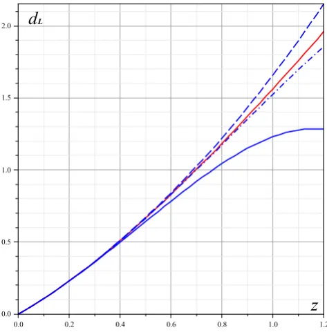
Figure 1.Comparison of the numerical solution to Eq. (9) for theΛCDM model (red line) with the approximate solutions given by (26) (blue solid line), (27) (blue dashed line), and (28) (blue dot-dashed line).

where the present magnitudes of the deceleration parame-terq = −a¨a/a˙2 _{and the jerk parameter}_j ₌ _a2..._{a /}_a_˙3 _are

denoted asq0andj0, respectively. By using (32), both

equa-tions (30) and (31) lead to the same expression forq0as

fol-lows

q0=−1 +

3

2Ωm. (33)

In the framework of this paper, we are not trying to con-strain parameters of this model with the observational data. For the illustrative purpose only, let us insertΩΛ = 0.72and

Ωm = 0.28in (29). Then we haveq0 ≈ −0.58, which is

within the observational limits.

Table 1.Percentage of relative errors of the corresponding approximations todLgiven by Eqs. (26), (27) and (28).

z % byd(1)_L % byd(2)_L % byd(3)_L 0.1 0.0989 0.00326 0.0001 0.2 0.4409 0.0301 0.0017 0.3 1.098 0.1153 0.0099 0.4 2.1457 0.3043 0.0363 0.5 3.6642 0.6497 0.1004 0.6 5.7351 1.2042 0.2318 0.7 8.4419 2.0118 0.4708 0.8 11.8697 3.0972 0.8678 0.9 16.1048 4.4579 1.4812 1.0 21.2349 6.0624 2.3729 1.1 27.3491 7.8615 3.6029 1.2 34.5383 9.8250 5.2277

With the help of Maple package, the graphs ofdL(z)in units ofc/H0 for the numerical solutions to the integral in

equation (9), and the approximate solutions (26) - (28) are shown in Fig. 1, where we have usedΩm = 0.28,ΩΛ =

0.72,Ωr = 0. Besides, Table 1 shows the percentage of re-lative errors of the approximate solutions compared to the numerical one.

For the next example, we consider a spatially flat universe with the quintessential matter. Let the equation of state pa-rameter be equals to−1 < wq < −1/3. Then equation (6) becomes as follows

W(z) = Ωm(1 +z)3+ Ωq(1 +z)3(1+wq), (34) which, being substituted in (26), yields

d(1)_L (z) =c(1 +z)

H0

₃

2z− Ωm

8

(1 +z)4−1

− 1−Ωm

2(4 + 3wq)

(1 +z)4+3wq₋₁

. (35)

Just as easy, the explicit expressions ford(2)_L (z)andd(3)_L (z)

can be obtained from equations (27), (28) and (34). The graphs of all approximations in this case are similar to those in Fig. 1, from which we could conclude that the first-order approximation may be useful only forz1. This is the ob-vious consequence of coincidence of (10) and (26) followed from the decomposition

1

p

W(z0₎ =

1

p

1 + (W(z0₎₋₁₎ ≈1−

1 2[W(z

0₎₋_1]_,

which can provide an acceptable accuracy only forz 1. Nevertheless, even the first-order approximation could be im-proved by some additional tuning. Let us consider an exam-ple of such a possibility.

Suppose that we want to improve the accuracy of the first-order approximation (26) in a vicinity of the point z = z0.

For this end, we can insert an indefinite parameterp1in

equa-tion (23), say, as follows

u1(z) =

3 2p z−

1 2(1−p)

z

Z

0

W(s)ds. (36)

At the same time, the exact expression foru(z)is given by (10) asu(z) =

z

R

0

ds

p

W(s). The necessary condition for the

minimum of difference betweenu(z)andu1(z)from (23),

that is

u(z)−u1(z) 0

|z=z0= 0, yields

p= 2 +W(z0)

p

W(z0)

[3 +W(z0)] p

W(z0)

. (37)

As an example, let us putz0 = 1, Ωm = 0.28andwq = −2/3in equations (29) and (34). One can obtain from (37) thatp≈0.7in both cases with different accuracy. Therefore, we have

d(Λ)_L (z) =c(1 +z)

H0

3

2p z−(1−p) Ωm

8 (1 +z)

4₋₁

+(1−p)1−Ωm 2 z

(6)

for theΛCDM model, and

d(_Lq)(z) = c(1 +z)

H0

₃

2p z−(1−p) Ωm

8

(1 +z)4−1

−(1−p)1−Ωm 4

(1 +z)2−1

,(39)

for the qCDM model withwq=−2/3.

z

0.0 0.2 0.4 0.6 0.8 1.0 1.2 1.4 0.0

0.5 1.0 1.5 2.0

z

[image:6.595.58.304.96.439.2]

d

L

Figure 2. Comparison of the numerical solution to Eq. (9) for theΛCDM model (black line) and qCDM model (blue line) with the approximate so-lutions given by (38) (red dot line) and (39) (green dot line), and the corre-sponding first-order approximations, (30) and (35) (dashed lines).

Table 2.Percentage of relative errors of the corrected approximations todL

given by Eqs. (38) and (39).

z % byd(Λ)_L % byd(_Lq) 0.70 1.4096 0.85718 0.75 0.9688 1.13112 0.80 0.5731 1.32456 0.85 0.2269 1.43455 0.90 0.0656 1.45812 0.95 0.3004 1.39219 1.00 0.4736 1.23365 1.05 0.5809 0.97930 1.10 0.6186 0.62589 1.15 0.5826 0.17009 1.20 0.4688 0.39144 1.25 0.2733 1.06216 1.30 0.0078 1.84559 1.35 0.3785 2.74519

Fig. 2 shows the corresponding numerical solutions of (9) for theΛCDM model (black solid line) and the qCDM mo-del (blue solid line) compared to the corresponding approx-imations (red and green lines, respectively). The dot lines represent the improved approximations given by equations

(38) and (39). The dashed lines represent the corresponding first-order approximations by equations (30) and (35).

The obvious advantage of the corrected approximations gi-ven by (38) and (39) becomes egi-ven more clear from Table 2, where we represent the percentage of relative errors provided by these equations. It can be readily concluded that the rela-tive errors of the simple approximations by (38) and (39) are mostly less then 1% for the redshift within the vicinity of 1. It can be assumed that an even more accurate approximations can be obtained by a similar method applied to the second-and third-order approximations.

6 Conclusions

Thus, a simple analytical computation of the luminosity distance in relativistic cosmology via the Variational Iteration Method has been considered. For this end, we have used the proposed earlier by the author conversion of the problem of calculating the integral in the well-known expression for the luminosity distance (8) to the problem of solving the Cauchy problem of the corresponding nonlinear differential equation (17). In this paper, the approximate solution of this equation is performed by using VIM in a direct way without using any restrictive assumption. Therefore, the computation becomes simple but rather effective, at least, in a vicinity of some value ofz. The relative accuracy of this method is briefly analyzed from the graphical representations of approximations obtai-ned, and the numerical evaluation of their relative errors. It would be noted that this method can be extended to cover the variety of cosmological models with different expressions for

W(z). This approximation seems to be useful in the models involvingW(z)in the form of non-polynomial over(1 +z)

expression.

REFERENCES

[1] A. G. Riess, et al. Observational Evidence from Super-novae for an Accelerating Universe and a Cosmological Constant, Astronomical Journal, Vol. 116, 1009, 1998. http://dx.doi.org/10.1086/300499

[2] S. Perlmutter, et al. Measurements of Omega and Lambda from 42 High-Redshift Supernovae, Astrophysical Journal, Vol. 517, 565, 1999. http://dx.doi.org/10.1086/307221

[3] N. Suzuki, D. Rubin, C. Lidman, et al. The Hubble Space Telescope Cluster Supernova Survey. V. Improving The Dark-Energy Constraints Abovez >1and Building an Early-Type-Hosted Supernova Sample, Astrophysical Journal, 746, 85, 2012.

[4] R. Amanullah, et al. Spectra and Light Curves of Six Type Ia Supernovae at0.511 < z < 1.12and the Union2 Com-pilation, Astrophysical Journal, Vol. 716, 712-738, 2010. http://dx.doi.org/10.1088/0004-637X/716/1/712

[image:6.595.101.255.545.712.2]

(7)

Dis-tance, Mon. Not. R. Astron. Soc., Vol. 412, 2685, 2011. http://dx.doi.org/10.1111/j.1365-2966.2010.18101.x

[6] Ce´line Cattoe¨n and Matt Visser. The Hubble series: con-vergence properties and redshift variables, Class. Quantum Grav., Vol. 24, 5985, 2007. http://dx.doi.org/10.1088/0264-9381/24/23/018

[7] Ue-Li Pen. Analytical Fit to the Luminosity Distance for Flat Cosmologies with a Cosmological Constant, Astrophys. J. Suppl. S., Vol. 120, 4950, 1999.

[8] Hao Wei, Xiao-Peng Yan, Ya-Nan Zhou. Cosmological Ap-plications of Pade Approximant,JCAP, Vol. 1401, 045, 2014. http://dx.doi.org/10.1088/1475-7516/2014/01/045

[9] A. Meszaros, J. Ripa. On the relation between the non-flat cosmological models and the elliptic integral of first kind, Astron. Astrophys., Vol. 573, A54, 2015. https://doi.org/10.1051/0004-6361/201425201

[10] J.-H. He. Homotopy perturbation technique,Computer Met-hods in Applied Mechanics and Engineering, Vol. 178, 257-262, 1999. http://dx.doi.org/10.1016/S0045-7825(99)00018-3

[11] V. K. Shchigolev. Calculating Luminosity Distance versus Redshift in FLRW Cosmology via Homotopy Perturbation Method, arXiv:1511.07459.

[12] V. Shchigolev. Homotopy Perturbation Method for Solving a Spatially Flat FRW Cosmological Model,Universal Jour-nal of Applied Mathematics, Vol.2, No. 2, 99-103, 2014. http://dx.doi.org/10.13189/ujam.2014.020204

[13] V. Shchigolev. Analytical Computation of the Perihe-lion Precession in General Relativity via the Homo-topy Perturbation Method, Universal Journal of Com-putational Mathematics, Vol. 3, No. 4, 45-49, 2015. http://dx.doi.org/10.13189/ujcmj.2015.030401

[14] V. K. Shchigolev, D. N. Bezbatko. On HPM approximation for the perihelion preces-sion angle in general relativity, Interna-tional Journal of Advanced Astronomy, Vol. 5, No. 1, 38-43, 2017. http://dx.doi.org/10.14419/ijaa.v5i1.7279.

[15] J.-H. He. Variational iteration method - a kind of non-linear analytical technique: some examples,International Journal of Non-Linear Mechanics, Vol. 34, No. 4, 699-708, 1999. http://dx.doi.org/10.1016/S0020-7462(98)00048-1

[16] J.-H. He. Variational iteration method for autonomous ordinary differential systems, Applied Mathematics and Computation, Vol. 114, No. 2-3, 115-123, 2000. http://dx.doi.org/10.1016/S0096-3003(99)00104-6

[17] J.-H. He. Variational iteration method-Some recent re-sults and new interpretations, Journal of Computational and Applied Mathematics, Vol. 207, No. 1, 3-17, 2007. http://dx.doi.org/10.1016/j.cam.2006.07.009

[18] V. K. Shchigolev. Variational iteration method for studying perihelion precession and deflection of light in General Rela-tivity,International Journal of Physical Research, Vol. 4, No. 2, 52-57, 2016. http://dx.doi.org/10.14419/ijpr.v4i2.6530 [19] M. Tatari and M. Dehghan. On the Convergence of He’s

Variational Iteration Method,Journal of Computational and Applied Mathematics, Vol. 207, No. 1, 121-128, 2007. http://dx.doi.org/10.1016/j.cam.2006.07.017

[20] J. I. Ramos. On the Variational Iteration Method and Other Iterative Techniques for Nonlinear Differential Equations, Ap-plied Mathematics and Computation, Vol. 199, No. 1, 39-69, 2008. http://dx.doi.org/10.1016/j.amc.2007.09.024

[21] Ernest Scheiber. On the Convergence of the Variational Itera-tion Method, arxiv:1509.01779.

[22] S. Weinberg,Gravitation and Cosmology: Principles and Ap-plications of The General Theory of Relativity(John Wiley. Press, New York, 1972).