Optimising manufacturing schedule using petri net

Full text

(1)Journal of Science and Technology UTHM. Optimising Manufacturing Schedule Using Petri Net. Sh Salleh bin Sh Ahmad Faculty of Mechanical and Manufacturing Enginereing Universiti Tun Hussein Onn Malaysia *Corresponding email: saleh@uthm.edu.my. Abstract The objective of this work is to propose an approach based on timed transition Petri net models to solve the scheduling problem of a manufacturing process. The approach uses process flow diagram to identify the main activities of the system and routings of the manufacturing work process. Based on the process flow diagram, corresponding timed transition Petri net models are produced and they are used for simulation purposes to determine the start and completion time at each work process. Petri net simulations are also used to determine the optimal schedule arrangement. Based on the Petri net simulations result, alternative makespan and completion time algorithms focusing on the bottleneck process in the manufacturing system are developed. These algorithms are found to be effective within specific limitation characteristics known as absolute bottleneck conditions.. 27. chap 3.indd 27. 12/13/2009 12:28:22 AM.

(2) Journal of Science and Technology UTHM. 1. IntroductIon Petri nets (PN) are known as a promising tool for describing and studying information processing systems that are characterised as being concurrent, asynchronous, distributed, parallel, nondeterministic, and/or stochastic [1]. They have been used to model real time system because they allow good representation of precedence constraints, conflict situations, shared resources and explicit quantitative time constraints in the timed PN case [2]. Many papers have reported the capability of PN theory as an efficient tool for modelling and analysis of operation scheduling activities. Scheduling of flexible manufacturing system using PN net was reported in [3] whereas Timing Constraint PN analysis and its application to schedulability analysis of real time system specifications were studied in [4]. This was followed in [5] that presented a model called Time Workflow Nets and associates time intervals with the transitions of the ordinary PN model. This work reported a case study in a health care system where a nurse who takes care of two patients is represented by a single token in a shared place. A verification technique of the schedulability of a workflow model was later proposed in [6]. A few researchers concentrated their effort on studying the capability of PN to model and analyse collaborative effort or inter-organisational work processes. Ling and Loke [7] reported how advanced PN techniques can be used to model mobile agent enabled inter-organisational workflows. In another research [8], PN was used to model a framework intended for distributed collaborative design environment which supports teamwork in an advanced CAD/CAM product development. Recently, finite scheduling of collaborative design and manufacturing activity using PN approach was reported in [9]. This paper focuses on utilising the PN to model, analyse and solve the activity scheduling problem of a design and manufacturing activity. It is intended to search for appropriate makespan algorithms, completion time algorithms and optimum solutions while describing the characteristic of the studied manufacturing environment. The process scheduling resembles a four machine manufacturing line with the processing route of M1,M2,M3,M4,M3,M4 in which the machine M3 is shared by the 3rd and 5th processes whereas the machine M4 is shared by the 4th and 6th processes. It was also noticed that in typical processes, the M1 and M4 always exhibiting bottleneck characteristics in which the longest or dominant processing time is always either from these two machines. However, this paper concentrates only on the scheduling analysis where the bottleneck is identified at M4. The remainder of the paper is organised as follows: Section 2 discusses basic Petri net components and their functions. This is followed with the modelling of the specific design and manufacturing activity in section 3 and scheduling analysis in section 4. Lastly, the two final sections discuss the makespan algorithms based on bottleneck process, summarise the findings and present the research conclusion.. 28. chap 3.indd 28. 12/13/2009 12:28:22 AM.

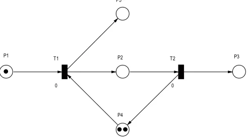
(3) Journal of Science and Technology UTHM. 2. BasIc PetrI net Petri net (PN) was introduced in 1962 by Carl A. Petri, who studied communication system for automation [10]. The findings were further developed by his successors especially in the area of process synchronization, asynchronous events, concurrent operations, and conflicts or resource sharing of industrial automated systems. Since 1970’s, engineering researchers started utilizing the PN to study and analyze manufacturing automation systems as the traditional continuous and discrete-time systems theory becomes insufficient to handle them. In describing PN, Proth and Xie [11] define it as a directed graph which has two types of nodes called places and transitions. The function of the directed arcs is to join places to transitions, or transitions to places. Directed arcs are not allowed to join places to places or transitions to transitions. Places are graphically represented by circles and transitions are pictured by rectangles or bars. Each place may contain none or a positive number of tokens represented by solid dots. Tokens are used to model the dynamics of the system. A simple example of a PN model is illustrated in Figure 1. In this example, places are identified as P1, P2, P3, P4 and P5 while transitions are denoted as T1 and T2. Its initial marking is the vector M0 = [1,0,0,2,0]. Normally, each arc is associated with a weight, which is a positive integer number. When the weight is not specified on the arcs, as illustrated in this example, it is assumed that the weight for all the arcs is equal to one. P5. P1. T1. P2. T2. 0. P3. 0. P4. Figure 1 : Example of PN Model. Formally, a PN is a five-tuple PN = (P, T, A, W, M0) where: P = {P1, P2, …., Pn} is a finite set of places, T = {T1, T2, …., Tm} is a finite set of transitions, A = is a finite set of arcs (places to transitions and transitions to places), W = is the weight function attached to the arcs, M0 = is the initial marking. A PN without marking is denoted by N = (P, T, A, W). As such the PN can be rewritten as PN = (N, M0). If all the weights are equal to 1, the PN is said to be ordinary. If M0 is the initial marking of a PN, then M0(P) is the number of tokens in the place P of the PN. Lets 29. chap 3.indd 29. 12/13/2009 12:28:22 AM.

(4) Journal of Science and Technology UTHM. consider the PN in Figure 1 and its initial marking M0 = [1,0,0,2,0]. Firing transition T1 leads to marking M1 = [0,1,0,1,1]. This is shown in Figure 2. If from this status, T2 is fired, the new marking M2 = [0,0,1,2,1] will be resulted as shown in Figure 3. In this case, it is said that M2 is reached from M0 by firing sequence σ = < T1, T2 >. This can be written as M0 M2 and sequence σ is said to be fireable. P5. P1. T1. P2. 0. T2. P3. 0. P4. Figure 2 : Status of the Example PN in Figure 1 After Firing T1 P5. P1. T1. P2. 0. T2. P3. 0. P4. Figure 3 : Status of the PN in Figure 2 After Firing T2. The inclusion of time in a PN model can be done in two different ways. The first method is done by attaching time to the transitions, resulting in a timed transition Petri net (TTPN). The other alternative is by attaching the time to the places, resulting in a timed place Petri net (TPPN). The delays in a timed Petri net (TPN) represent temporal restrictions. In a TPPN, when a token is put in a place Pi, it remains unavailable for a time equal to the delay time attached to Pi, after which only it becomes available [12]. Only available tokens in a marking can enable a transition. If a transition is attached by a time delay as in TTPN, this means that the token generated due to the firing of the transition has to spend a processing time equivalent to the value of the attached delay time before reaching the next intended place [10]. 30. chap 3.indd 30. 12/13/2009 12:28:22 AM.

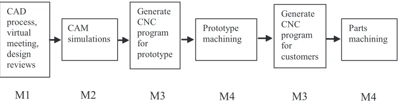
(5) Journal of Science and Technology UTHM. 3. desIgn and ManufacturIng actIvIty ModellIng The first step in developing the PN model of the design and manufacturing activity is to establish a process flow that described all activities related to the system. The overall process flow at the system is illustrated in Figure 4. The process flow consists of six major tasks. The first task consisting of CAD process, virtual meeting and design reviews are conducted at a dedicated workstation identified as M1 while the second tasks involving the CAM simulation is done at workstation M2. The third task (generate CNC program for prototype) and the fifth task (generate CNC program for customer) shares a common CNC post-processor indicated as M3. The fourth task (prototype machining) and the final task (parts machining) also shares a common CNC machine identified as M4. Using the workstations and machine identification, the process routing can be written as M1, M2, M3, M4, M3 and M4. This means that a job going through the process route will have to re-enter M3 and M4 for its fifth and sixth process. Another constraint that appears in the process environment is that the queues in front of each work station or machine operate according to the First In First Out (FIFO) rule. This means that the order in which the jobs go through the first workstation is maintained throughout all other workstations and a job cannot “overtake” other jobs while waiting in a queue. This type of flow shop is known as a permutation flow shop. Since all jobs have to follow exactly the permutation rule and the same process flow or route that involves re-entry, therefore the scheduling problems at the design and manufacturing process fall under the category of permutation re-entrant flow shop. Other than re-entry, the activities also exhibit the tendency of bottleneck characteristics at M1 and M4.. CAD process, virtual meeting, design reviews. CAM simulations. Generate CNC program for prototype. M1. M2. M3. Prototype machining. M4. Generate CNC program for customers. Parts machining. M3. M4. Figure 4: Design and manufacturing activity process flow. The conceptual PN model that illustrates the overall activities of the studied manufacturing system is shown in Figure 5. This PN model was developed using Visual Object Net ++ software version 2.0a. From the model, it can be seen that all jobs must visit the work centres in the same sequence. This is similar with flow shop manufacturing as described in [13,14]. It can also be noticed that both shared resources (P24 and P25) must completely finish the processing of a particular job at T5 and T6 31. chap 3.indd 31. 12/13/2009 12:28:22 AM.

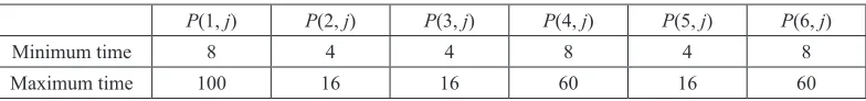
(6) Journal of Science and Technology UTHM. before starting to process any new job at T3 and T4. In other words, the PN model matches the description of four machine permutation re-entrant flow shop with the routing of M1,M2,M3,M4,M3,M4.. P1. C A D de sig n, virtua l m e e ting , d esig n re vie w T1 P2. G e ne ra te C N C p rog ra m fo r p ro totype T3. CAM sim u la tion T2. 15. P3. 3. P ro totype m a ch in in g T4. P4. 2. G e ne ra te C N C p rog ra m fo r cu sto m e r T5. P5. 8. P6. 2. T6. P7. 16. P24 P22. P a rts m a ch in in g. P25. P23. C A D syste m. C A M syste m. C N C p o stp ro ce sso r. C N C m a ch ine. (M 1 ). (M 2 ). (M 3 ). (M 4 ). Figure 5 : PN model for process activity [15]. 4. schedulIng analysIs Let say, the manufacturing system is currently having four jobs that need to be processed. Typical processing time ranges for all processes are shown in Table 1. P(1, j) to P(6, j) represents the process time for the first to the last processes. These time ranges are then used to generate random data for the four jobs that need to be processed. The randomly generated data is shown in Table 2. All the data are then used to build a PN model representing all job activities at the system. Assuming that the data in Table 2 is arranged in the order of First-come-first-served (FCFS) basis, then the PN model representing a FCFS scheduling arrangement is illustrated in Figure 6. Table 1 : Processing time range (hr) P(1, j). P(2, j). P(3, j). P(4, j). P(5, j). P(6, j). Minimum time. 8. 4. 4. 8. 4. 8. Maximum time. 100. 16. 16. 60. 16. 60. Table 2 : Processing time data (hr) P(1, j). P(2, j). P(3, j). P(4, j). P(5, j). P(6, j). Job A. 14. 5. 8. 9. 7. 17. Job B. 33. 8. 4. 9. 7. 28. Job C. 38. 8. 4. 39. 4. 11. Job D. 15. 4. 5. 21. 5. 15. 32. chap 3.indd 32. 12/13/2009 12:28:22 AM.

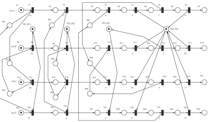
(7) Journal of Science and Technology UTHM. T1. P1. T2. P2. T3. P3. T4. P4. T5. P5. T6. P6. P7. Job A 14 P26. 5. 8. P61. P22 (R1). 9. 7. 17. P62. P24 (R3) P23 (R2). P8. T8. T9. P9. P25 (R4). T10. P10. T11. P11. T12. P12. T13. P13. P14. Job B 33. 4. 8. T15. P15. 9. 28. 7. P65. P64. P27. T16. P16. P18. T17. P17. T18. T19. P19. P21. T20. P20. Job C 38. P28. 4. 8. 39. P68. 4. 11. P67. T30. P30. T29. P29. T31. P31. T32. P32. T33. P33. T34. P34. P35. Job D 15. 5. 4. 21. 5. 15. Figure 6 : PN model of first-come-first-served schedule arrangement. This research utilizes the Integrated Net Analyser (INA) version 2.2 to analyse the PN model in order to obtain the makespan. This is achieved by using a built-in function for searching the shortest path from initial marking to a target marking. The target marking is set to be for P7, P14, P21 and P35 to have one token at each place. The results indicate that the makespan for the FCFS arrangement is 199 hours. In order to allow INA to search for an optimum job arrangement, the PN model in Figure 6 has to be modified. This modification is shown in Figure 7. T50. P50. Job A. T1. P1. 0. T71. P2. 14. Job B. P52. Job C. P53. Job D. T51. T8. P8. 0. T52. 0. T15. P16. 38. 0. T53. P9. 33. P15. P29. T72. T29. 15. T79. T78. P77. 0. P78. T83. P83. T84. P84. 0. 0. T85. 0. P89. T90. 0. T9. P85. T16. 0. P90. T91. 0. T30. P10. P17. T76. P76. 0. P64. T3. T4. P4. 8. T5. P5. 9. P6. 7. T6. P7. 17. P24 (R3). T81. T80. 0. P80. 0. T86. P86. T87. T92. P92. P81. 0. T93. 0. T10. T82. P87. 0. P82. 4. T88. P88. T17. 0. 0. P31. 4. P75. 0. P25 (R4). 8. P91. T75. P63. 8. P79. P74. 0. P23 (R2). 0. T89. T74. P3. 5. P62. T77. T2. P73. T73. 0. 0. P30. P72. 0. P61. P22 (R1). P51. P71. 0. P93. T94. 0. P94. T31. 5. T12. P12. 9. P18. 4. 0. T11. P11. 39. P32. T32. T19. P19. P20. 4. P33. 21. T33. 5. P14. 28. 7. T18. T13. P13. T20. P21. 11. P34. T34. P35. 15. Figure 7 : PN model for searching the optimum job arrangement. 33. chap 3.indd 33. 12/13/2009 12:28:22 AM.

(8) Journal of Science and Technology UTHM. T1. P1. T2. P2. T3. P3. T4. P4. T5. P5. T6. P6. P7. Job A 14. 5. 8. P61. P26. P62. 7. 17. P24 (R3). P23 (R2). P22 (R1). 9. P25 (R4). P8. T8. T9. P9. Job B 33. T12. P12. 9. P14. T13. P13. 28. 7. P65. P16. T15. T11. P11. 4. 8 P64. P27. P15. T10. P10. T16. P18. T17. P17. T19. P19. T18. P21. T20. P20. Job C 38. P28. 8. 4. P68. 39. 4. 11. P67. P29. P30. T29. T30. T31. P31. T32. P32. P33. T33. T34. P34. P35. Job D 15. 5. 4. 21. 5. 15. Figure 8 : PN model for optimum job arrangement with DACB job sequence. INA is then used to search for shortest path from initial marking of Figure 7 to a target marking of one token each at P7, P14, P21 and P35. The results indicate that the minimum makespan is 196 hours with the job sequence of DACB. Visual Object Net ++ was used to obtain the completion time of each process for all the jobs with this optimum arrangement by simulating the model at Figure 8. This data is then used to determine the start and stop time of each process as shown in Table 3. Table 3 : Start and stop time for each task with DACB job sequence P(1, j) Start. Stop. P(2, j) Start. Stop. P(3, j) Start. Stop. P(4, j) Start. Stop. P(5, j) Start. Stop. P(6, j) Start. Stop. Job D. 0. 15. 15. 19. 19. 24. 24. 45. 45. 50. 50. 65. Job A. 15. 29. 29. 34. 50. 58. 65. 74. 74. 81. 81. 98. Job C. 29. 67. 67. 75. 81. 85. 98. 137. 137. 141. 141. 152. Job B. 67. 100. 100. 108. 141. 145. 152. 161. 161. 168. 168. 196. Referring to Table 2 and Table 3, the scheduling algorithm for the manufacturing system can be written as the followings and is identified as Algorithm 1 [9]: Algorithm 1 Let i = Task number, process sequence or work centre number ( i = 1, 2, 3, ….) j = Job number ( j = 1, 2, 3, ….). 34. chap 3.indd 34. 12/13/2009 12:28:23 AM.

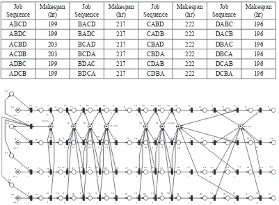
(9) Journal of Science and Technology UTHM. Start ( i, j ) = start time of the jth job at ith process. Stop ( i, j ) = stop time of the jth job at ith process. P ( i, j ) = processing time of the jth job at ith process. For i = 1, 2, 5, 6 and j = 1, 2, 3,… Start ( i, j ) = Max [Stop (i, j-1), Stop ( i-1, j )] except Start (1, 1) = initial starting time Stop ( i, j ) = Start ( i, j ) + P ( i, j ) For i = 3, 4 and j = 1, 2, 3,…. Start ( i, j ) = Max [Stop ( i, j-1 ), Stop ( i-1, j ), Stop ( i+2, j-1 )] Stop ( i, j ) = Start ( i, j ) + P ( i, j ) Using Algorithm 1, the start and stop times for processes belong to ABCD job sequence are computed. The makespan for ABCD job sequence is 199 hours which is indicated by the stop time of the last task belongs to the last job. The makespan for all other possible job sequences representing ABDC, ACBD and others were also computed. This is shown in Table 4. In order to ascertain the accuracy of Algorithm 1, a PN model that allows the user to arrange the job sequence is drawn and Visual Object Net was used to determine the makespan for each job sequence arrangement. This PN model is illustrated in Figure 9. In this PN model, the arc weightings written between P54-T50, P55-T51, P56T52 and P57-T53 are the sequence selected for the individual job. The example in Figure 9 illustrates the job sequence of DABC. Since there are a total of four jobs to be arranged, therefore there will be 4 factorial (4!) or 24 different sequence arrangements. The results of all the makespan analysis by Visual Object Net are illustrated in Table 5. Since all the makespan values in Table 4 are the same with the makespan in Table 5, this indicates the Algorithm 1 is accurate in computing the makespan for the studied manufacturing system scheduling. Table 4 : Makespan from different job sequences using Algorithm 1 Job Sequence. Makespan (hr). Job Sequence. Makespan (hr). Job Sequence. Makespan (hr). Job Sequence. Makespan (hr). ABCD. 199. BACD. 217. CABD. 222. DABC. 196. ABDC. 199. BADC. 217. CADB. 222. DACB. 196. ACBD. 203. BCAD. 217. CBAD. 222. DBAC. 196. ACDB. 203. BCDA. 217. CBDA. 222. DBCA. 196. ADBC. 199. BDAC. 217. CDAB. 222. DCAB. 196. ADCB. 199. BDCA. 217. CDBA. 222. DCBA. 196. 35. chap 3.indd 35. 12/13/2009 12:28:23 AM.

(10) Journal of Science and Technology UTHM. Table 5 : Makespan from different job sequences using Petri net Job Sequence. Makespan (hr). Job Sequence. Makespan (hr). Job Sequence. Makespan (hr). Job Sequence. Makespan (hr). ABCD. 199. BACD. 217. CABD. 222. DABC. 196. ABDC. 199. BADC. 217. CADB. 222. DACB. 196. ACBD. 203. BCAD. 217. CBAD. 222. DBAC. 196. ACDB. 203. BCDA. 217. CBDA. 222. DBCA. 196. ADBC. 199. BDAC. 217. CDAB. 222. DCAB. 196. ADCB. 199. BDCA. 217. CDBA. 222. DCBA. 196. P54. 2. T50. P50. Job A. P55. T1. P1. 0. 14. T54. P22 (R1). T71. P2. P71. T72. P72. 0. 0. T74. P3. 5. 0. P61. T2. P73. T73. P62. P74. T75. P75. 0. P63. P23 (R2). T76. P76. 0. 0. P64. T3. T4. P4. 8. T5. P5. 9. P6. 7. T6. P7. 17. P24 (R3) P25 (R4). 0 3 P51. T51. T8. P8. 0. Job B. P9. 33. T79. T78. T77. 0. P77. 0. P78. T83. P83. T84. P84. 0. T9. P10. 8. P79. T81. T80. 0. P80. 0. T86. P86. T87. T10. T82. P81. 0. P82. 4. T88. P88. T17. T11. P11. T12. P12. 9. T13. P13. P14. 28. 7. P56. 4 P52. Job C. T52. P15. T15. P16. 38. 0. T85. 0. 0. T16. P85. 0. P17. 8. P87. 0. 0. P18. T18. 4. 0. T19. P19. 39. P20. 4. T20. P21. 11. P57. P53. Job D. 1. T53. 0. P29. T29. 15. P30. T89. 0. P89. T90. 0. P90. T91. 0. P91. T30. P31. 4. T92. 0. P92. T93. 0. P93. T94. 0. P94. T31. P32. T32. 5. 21. P33. T33. P34. 5. T34. P35. 15. Figure 9 : PN model for user selected job sequence. 5. MakesPan algorIthM focusIng on M4 as the Bottleneck Process From Table 4 and Table 5 (discussed in section 4), it can be seen that the minimum makespan is achieved by arranging Job D as the first job. The second, third and last job can be assigned to any other jobs without affecting the makespan value. The maximum makespan is achieved by arranging Job C as the first job. It can also be noticed from the results that a vast majority of the makespan value is influenced by the assignment of the first job. Almost all scheduling sequence that begins with the same job will result to the same makespan value. The only exception is the scheduling sequence of ACBD and ACDB which produces higher makespan than other sequence that starts with Job A as the first job. In order to explain the behaviour of all the scheduling sequences from Table 4 and Table 5, detail studies were conducted on all the 24 different job arrangements. The Gantt charts of all job arrangements were compared and investigated for similarity and differences of 36. chap 3.indd 36. 12/13/2009 12:28:23 AM.

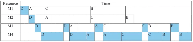
(11) Journal of Science and Technology UTHM. characteristics. From the observations, the makespan computation can be summarised as follows: For the job sequences which begin with A, B, C or D as the first job (AXXX, BXXX, CXXX or DXXX), excluding ACXX, the makespan calculation is: n. 3. 6. Cmax = ∑ P(i, 1) + ∑ ∑ P(i, j) i=1. j=1 i=4. (Equation 1) [9]. The example of the scheduling Gantt chart representing DACB job sequence is shown in Figure 10. It can be noted from this Gantt chart that M4+M3+M4 or {P(4,j) + P(5,j) + P(6,j)} is always the bottleneck of the scheduling system. Referring back to the processing time data in Table 2, the most dominant or bottleneck machine is identified as the M4. However, due to the re-entrant nature of the studied manufacturing system, the analysis utilises M4+M3+M4 P(i,j) in. as the bottleneck component. The bottleneck is represented by the value of. P(i,j) will always result to the same value at any job sequence,. Equation 1. Since. then the makespan is directly influenced by {P(1,1) + P(2,1) + P(3,1)} which is actually the sum of the first, second and third processing time for the job assigned as the first job. Equation 1 has similarity with the concept of completion time algorithm described in [16, 17] for the increasing dominant machine (idm) problem Fm|idm|γ. Resource M1 D M2 M3 M4. A. C. B. D. A. C. D. D A D. D. Time B A. A. C A. C B C. C. B B. B. Figure 10 : Scheduling Gantt chart for DACB job sequence (resource focused). Detail observation of Equation 1 suggests that this equation works well for makespan computation under strict bottleneck conditions. The conditions are meant to ensure that the processes of P(4,j) + P(5,j) + P(6,j) are always the bottleneck. This characteristic is identified as absolute bottleneck in which regardless of any job sequence arrangement, P(4,j) + P(5,j) + P(6,j) without fails are always the schedule bottleneck. The absolute bottleneck conditions related to Equation 1 are written as the followings: Max{j=1…n}[P( 3, j )] ≤ Min{j=1…n}[P( 6, j )]. (Condition 1). Max{j=1…n}[P( 2, j ) + P( 3, j )] ≤ Min{j=1…n}[ P( 3, j ) + P( 4, j ) + P( 5, j ) + P( 6, j )]. (Condition 2). Max{j=1…n}[P( 1, j ) + P( 2, j ) + P( 3, j )] ≤ Min{j=1…n} [ P( 2, j ) + P( 3, j ) + P( 4, j ) + P( 5, j ) + P( 6, j )]. (Condition 3). 37. chap 3.indd 37. 12/13/2009 12:28:23 AM.

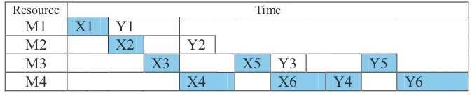
(12) Journal of Science and Technology UTHM. Condition 1, 2 and 3 are meant to ensure that no matter how the jobs are arranged, task 4 of a job (Y4 in Figure 11) can always begin immediately after the completion of task 6 of the immediate preceding job (X6). This means that for a job X starting on task 2, and job Y starting at task 1 at the same time, these conditions guarantee that job Y is always ready to begin its task 4 process immediately after job X releases the M4 machine for its task 6. Figure 11 shows this description in which Y4 can begins immediately after the completion of X6. Resource. M1 M2 M3 M4. X1. Y1 X2. Time. X3. Y2 X4. X5. Y3 X6. Y4. Y5. Y6. Figure 11 : Example schedule that fulfils Condition 1, 2 and 3. The explanations above indicate that Equation 1 will produce accurate makespan computation result if Condition 1, Condition 2 and Condition 3 were met. In order to test this statement, a total of 10000 simulations for four job sequence were conducted using random data between 1 to 20 hours for each of P(1,j), P(2,j), P(4,j), P(5,j) and P(6,j). The value of P(3,j) were set to be between 1 to 10 in order to have a more evenly distributed matching of either Condition 1, Condition 2, and Condition 3 or any of their combinations. Group of four jobs were chosen for the simulations because small job size permits a complete evaluation of all the possible job arrangements within a set of data. Each set of random data obtained was tested with a total of 24 different sequences that resemble the sequence arrangements of ABCD, ABDC, ACBD etc. This means that with 10000 simulations, a total of 240,000 job sequence arrangements were tested. The makespan results from using Equation 1 were compared with the makespan value obtained from Algorithm 1. In this analysis, a perfect result means that the makespan value computed using Equation 1 for all the twenty four job sequences from a set of four jobs data equal the result from Algorithm 1. The results from the simulations are summarised in Table 6. In this table, the percentage of perfect result is computed by obtaining the ratio of the perfect results data set against the total data sets belonging to each conditions criterion. The result shows that all makespan value from both Equation 1 and Algorithm 1 are equal for random data sets that fulfil all the three conditions. This indicates that Equation 1 is accurate for computing the makespan if Condition 1, Condition 2 and Condition 3 were met. With all these three conditions met, we can conclude that P( 4, j ) + P( 5, j ) + P( 6, j ) or the M4 machine processes are the absolute bottleneck of the scheduling system.. 38. chap 3.indd 38. 12/13/2009 12:28:23 AM.

(13) Journal of Science and Technology UTHM. Table 6 : Accuracy of Equation 1 at various conditions Conditions Met. Sets of Data Match The Conditions. Percentage of Perfect Result. 1+2+3. 1168. 100. 1+2. 333. 4.50. 1+3. 55. 23.64. 2+3. 3449. 4.26. 1. 162. 1.23. 2. 1893. 0.26. 3. 511. 0.98. -. 2429. 0. If a set of scheduling data fulfils the absolute bottleneck Condition 1, 2 and 3, then Equation 1 can be used to calculate the schedule makespan as well as to find the job sequences that provide the optimum makespan. The optimum makespan is achieved by assigning the first job sequence to the job that has the smallest value of {P(1,j) + P(2,j) + P(3,j)}. Furthermore, strictly depending on the job sequence, the completion time for each job (Cj) then can be computed as the followings: j. 3. 6. Cj = ∑ P(i,1) + ∑ ∑ P(i,k) i=1. (Equation 2). k=1 i=4. To illustrate the usage of Equation 1 and 2, the data that fulfils Condition 1, 2 and 3 in Table 7 is used to compute the makespan for the scheduling sequence of ABCD. This scheduling sequence is shown by the sequence arrangement at column j. The makespan computation using Equation 1 is: {P(1,1) + P(2,1) + P(3,1)} + {P(4,1) + P(5,1) + P(6,1) + P(4,2) + P(5,2) + P(6,2) + P(4,3) + P(5,3) + P(6,3) + P(4,4) + P(5,4) + P(6,4)} = {14 + 3 + 3} + {26 + 5 + 33 + 18 + 5 + 46 + 10 + 4 + 20 + 51 + 5 + 51} = 299 Table 7 : Processing Time (P( i, j )) (hr) Job. j. P( 1, j ). P( 2, j ). P( 3, j ). P( 4, j ). P( 5, j ). P( 6, j ). Job A. 1. 14. 3. 3. 26. 5. 33. Job B. 2. 10. 7. 8. 18. 5. 46. Job C. 3. 9. 6. 8. 10. 4. 20. Job D. 4. 18. 4. 3. 51. 5. 51. 39. chap 3.indd 39. 12/13/2009 12:28:24 AM.

(14) Journal of Science and Technology UTHM. The optimum makespan is achieved by assigning the first job sequence to the job that has the smallest value of {P(1,j) + P(2,j) + P(3,j)} which is job A. Therefore the optimum schedules are any job arrangements that begin with job A. The optimum makespan is equal to the makespan of ABCD job arrangement, 299 hours. Using Equation 2, the completion time of Job C during the execution of ABCD job arrangement is: {P(1,1) + P(2,1) + P(3,1)} + {P(4,1) + P(5,1) + P(6,1) + P(4,2) + P(5,2) + P(6,2) + P(4,3) + P(5,3) + P(6,3) = {14 + 3 + 3} + {26 + 5 + 33 + 18 + 5 + 46 + 10 + 4 + 20} = 187 hours. 6. conclusIons Accurate and effective scheduling is very important in manufacturing industries. In order to achieve this, the overall activities of the operation processes must be correctly modelled and analysed. This research presented an approach of utilizing PN to model a case study consisting of design and manufacturing activity. The PN models developed were: PN models representing FCFS, PN model for searching the optimum job arrangement, PN model to obtain the completion time of each process and PN model for user selected job sequence. These PN models were simulated to obtain completion time and makespan data for various job arrangements. Based on the simulation results, Algorithm 1 which is capable to compute the start and stop time for every process within a specified schedule arrangement was developed. An alternative makespan equation focusing on the identified bottleneck process was also introduced. This alternative makespan equation is found to be valid and effective within very specific limiting conditions known as absolute bottleneck conditions. If sets of data fulfil the absolute bottleneck conditions, the alternative makespan equation can be used to compute the makespan and to suggest for optimal job sequences. This approach can economically be studied and implemented since the PN software utilised can be obtain from the Internet without charges. As a conclusion, this paper has demonstrated a feasible application of PN in modelling a design and manufacturing activity case study. The PN model is found to be very useful in analysing the activity scheduling which also resembles a re-entrant flow shop or production line with shared resources. Similar modelling and scheduling approach is also applicable to ordinary flow shops operation such as in metal fabrications, furniture manufacturing and also machinery assemblies. However, activities involving larger number of processes will require larger and more complex PN model. A challenge for future research would then be to develop appropriate PN technique for solving complex scheduling problems.. 40. chap 3.indd 40. 12/13/2009 12:28:24 AM.

(15) Journal of Science and Technology UTHM. acknowledgeMents This work was partially supported by the Fundamental Research Grant Scheme, Ministry of Higher Education, Malaysia (Cycle 1 2007 Vot 0368).. references [1] Murata, T. (1989). Petri nets: properties, analysis and application. Proceeding of IEEE vol. 77(4), pp. 541-580 [2] Julia, S., Francielle de Oliveira, F. and Valette, R. (2008). Real time scheduling of workflow management systems based on a p-time Petri net model with hybrid resources. Simulation Modelling Practice and Theory, vol. 16, pp. 462-482 [3] Lee, D.Y. and DiCesare, F. (1994). Scheduling flexible manufacturing systems using Petri nets and heuristic search. IEEE Transactions on Robotics and Automation, vol. 10(3), pp. 123-132 [4] Tsai, J.J.P., Yang, S.J. and Chang Y.H. (1995). Timing constraint Petri nets and their application to schedulability analysis of real time system specifications, IEEE Transactions on Software Engineering. Vol. 21(1), pp. 32-49 [5] Ling, S. and Schmidt, H. (2000). Time Petri nets for workflow modelling and analysis. IEEE Transactions on Systems, Man and Cybernetics. pp. 3039-3044 [6] Li, J., Fan, Y. and Zhou, M. (2003). Timing constraint workflow nets for workflow analysis. IEEE Transactions on Systems, Man and Cybernetics. Part A: Systems and Humans, vol. 33(2) [7] Ling, S. and Loke, S. W. (2002). Advanced Petri Nets for Modeling Mobile Agent Enabled Interorganizational Workflows, Proceedings of the 9th Annual IEEE International Conference and Workshop on the Engineering of Computer-Based Systems (ECBS’02) [8] Ding, Y.F., Yang, F., Sheng, B.Y. and Zhou, Z.D. (2005). The Design and Realization of Automotive Steering Gear Collaborative Design System Based on Multi-Agent, Proceedings of the 4th International Conference on Machine Learning and Cybernetics, Guangzhou, vol. 1, pp. 276-281 [9] Bareduan, S. A., Hasan, S.H. and Ariffin, S. (2008). Finite Scheduling of Collaborative Design And Manufacturing Activity: A Petri Net Approach. Journal of Manufacturing Technology Management, vol. 19(2), pp. 274-288. [10] Zhou, M. C. and Jeng, M. D. (1998). Modeling, Analysis, Simulation, Scheduling, and Control of Semiconductor Manufacturing System: A Petri Net Approach. IEEE Transactions on Semiconductor Manufacturing, vol. 11(3), pp. 333-357 [11] Proth, J. M. and Xie, X. (1996). Petri Nets: A Tool for Design and Management of Manufacturing System, West Sussex, England: John Wiley. [12] Desrochers, A. A. and Al-Jaar, R. Y. (1995). Application of Petri Nets in Manufacturing Systems: Modeling, Control, and Performance Analysis, New York: IEEE Press. 41. chap 3.indd 41. 12/13/2009 12:28:24 AM.

(16) Journal of Science and Technology UTHM. [13] Onwubolu, G.C. (1996). A Flow-shop Manufacturing Scheduling System With Interactive Computer Graphics, International Journal of Operations & Production Management, vol. 16(9), pp. 74-84 [14] Pinedo, M. (2002). Scheduling: Theory, Algorithms, and Systems, New Jersey: Prentice-Hall [15] Bareduan, S. A.and Hasan, S.H. (2008). Bottleneck-Based Makespan Algorithm For Cyber Manufacturing System. Proceedings of International Conference on Mechanical & Manufacturing Engineering (ICME2008), Johor Bharu [16] Ho, J.C. and Gupta, J.N.D. (1995). Flowshop Scheduling With Dominant Machines. Computers and Operations Research, vol. 22(2), pp. 237-246. [17] Cepek, O., Okada, M. and Vlach, M. (2002). Nonpreemptive Flowshop Scheduling With Machine Dominance. European Journal of Operational Research. vol. 139, pp. 245-261.. 42. chap 3.indd 42. 12/13/2009 12:28:24 AM.

(17)

No results found