An Advanced Genetic Approach for Stacking Classifiers

2016 International Conference on Artificial Intelligence: Techniques and Applications (AITA 2016) ISBN: 978-1-60595-389-2

An Advanced Genetic Approach for Stacking Classifiers

Zhi-quan QIN

, Chang-jian WANG, Yu-xing PENG and Yuan YUAN

College of Computer, National University of Defense Technology, Changsha 410073, China *Corresponding author

Keywords: Classification, Ensemble, Stacking, Configuration selection, Genetic algorithm.

Abstract. A key to obtain a high quality of stacking ensemble is to select a proper configuration for the specific dataset. Various approaches are proposed on this topic. GA-Ensemble is an effective approach using genetic algorithm to select the configuration. However, the weakness of the problem encoding and the reproduction of unnecessary individuals in GA-Ensemble impact the accuracy of the approach. In this work, the subspace partition and a tabu strategy are used to improve the accuracy of GA-Ensemble. The results over 13 UCI datasets show that the new proposed approach has a better performance.

Introduction

Stacking is one of classic ensemble methods, it has been applied in various fields[1,2,3,4] and performs well in several data mining competitions[5,6]. With the learning combination, stacking is usually constructed of two levels of classifiers. The classifier in the low (base) level is called the base classifier and in the high (meta) level is called the meta classifier.

One problem of stacking is how to select a proper configuration of stacking, i.e., the combination of base classifiers and meta classifier. Both of the base and meta classifiers are considered in this problem. The size of the search space is𝑚 × 2𝑏− 1 if there are m candidate learning algorithms for the meta classifier and b candidate base classifiers. Exhaustive search, with no doubt, would cause a large cost of time and is impractical. In the earlier years, researchers used fixed configurations for classification[7,8,9,10]. But the results were ragged over multiple datasets because the configuration selection is domain specific. In recent years, researchers introduced heuristic search algorithms such as Genetic Algorithm[11] (GA) and Ant Colony Optimization[12] (ACO) to solve this problem and achieved great results. GA-Ensemble[13] (GA-E) is a simple and efficient approach using GA for the configuration selection. However, the encoding of the individual in GA-Ensemble underestimates the importance of the meta classifier, which lowers the quality of the search process. And when there are more than 2 candidates in the meta level, the limitation of the encoding may cause a loss of a better solution[14]. Besides, there are a number of reproductions of the unnecessary individuals, which takes up the chance of searching better configurations when the search space is not huge but still cost a lot of time.

In this paper, we propose an approach called Advanced GA-Ensemble (AGA-E) to improve the accuracy of GA-E. This new approach selects the configuration by several independent GA processes on subspaces and uses a tabu strategy to deal with the unnecessary reproduction. Empirical results on 13 UCI datasets shows that AGA-E is more adaptive and promising.

The structure of this paper is as follows. Section “Related Work” presents the related work of the configuration selection of stacking. Section “Advanced GA-Ensemble” gives the detailed description of the new proposed approach. In Section “Experiments and Results”, the experiments are described and the results are discussed. In Section “Conclusion and Future work”, the conclusion and future work are discussed.

Related Work

ensemble. In [8], the stacking using a modified decision tree as the meta classifier is proposed. In [9], StackingC, a variant of stacking with MLR, is proposed for multi-class classification. In [10], the stacking with Multi-Response Model Tree (MRMT) is proposed and it was concluded that the stacking with MRMT outperformed to the other variants above. However it is the combination of the meta and base classifiers that decides the performance and these variants of stacking only consider a part of it. And the results of the above work are unconvincing[16].

The heuristic search algorithms are introduced for the selection of the configuration. In [16], GA-Stacking which uses the GA to select the dataset dependent configuration is proposed. It selects the combination and the parameters of the classifiers. The authors concluded that it was comparable to the best reported results of fixed configurations but suffered from a long execution time. In [13], GA-Ensemble is proposed to improve the efficiency of GA-Stacking by using a pool of trained base candidates and reducing the meta candidates to 2 which, as mentioned before, lowers the quality of the output. In [14], ACO-Stacking is proposed, using the ACO to find the configuration.

Advanced GA-Ensemble

Extensionof GA-Ensemble

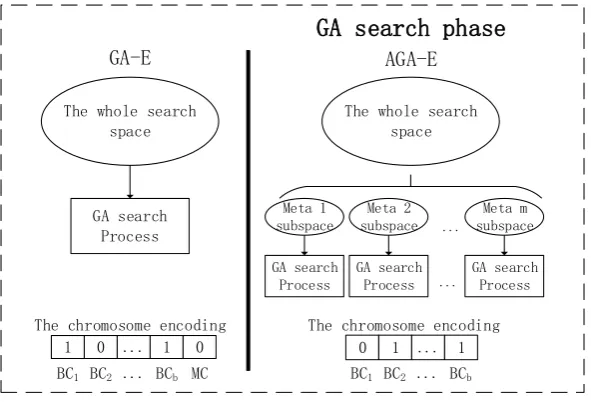
As mentioned before, the base classifiers and the meta classifier are the two important parts of the configuration, the meta part has the importance as much as the base part, i.e., 50%. The results of above work confirms that the configurations with the different meta classifier but the same base classifiers have different performances. For the analysis, we divide the whole search space into m

subspaces by the meta classifier at first.

Figure 1. The differences of GA-E and AGA-E.

Firstly, an individual in GA-E are represented by a chromosome with b bits of base genes and 1 bit of meta gene. However, the genes in the chromosome are treated equally. Therefore, the meta importance is 1/b of the base one, which means the genetic operations such as mutation, on subspaces happen as b times as the ones cross subspaces. Secondly, as a result of canonical binary encoding, GA-E can’t search the rest b-2 subspaces when b>2. These two points make GA-E a weak search ability cross the subspaces and lowers the quality of the selected configuration.

Therefore, the encoding mixing the base and meta genes is not suit for the selection problem in stacking. And then we extend the GA-E by running m independent GA search processes like GA-E on subspaces (Figure 1). So AGA-E has the same search ability on each subspace and can handle the situation of multiple meta candidates. The size of chromosome is b in the processes instead of b+1 in GA-E. The GA search process goes to select a best individual on each subspace. The selected individual and its configuration are called local best individual and local best configuration (LBC)

The whole search space

The whole search space

GA search Process

GA-E AGA-E

GA search phase

...

...

The chromosome encoding

Meta 1 subspace

Meta 2 subspace

Meta m subspace

GA search Process

GA search Process

GA search Process

1 0 ... 1 0 The chromosome encoding

BC1 BC2 ... BCb MC

respectively. At the end of AGA-E, the LBC with the highest individual fitness is chosen as final configuration.

Strategyfor the Reproduction

It is pointed out that GA-E lacks strategies for the reproductions of the weak individuals[14]. Inspired by this point, we think that there are also some reproductions of unnecessary individuals. These individuals are not the global optima but have a relatively high fitness and therefore are reproduced with a quite probability in the evolution of population. Because of the limited size of population, using the places the unnecessary individuals occupy to search the new space can improve the chance of finding good configurations and the effectiveness of the search.

Figure 2. The GA process.

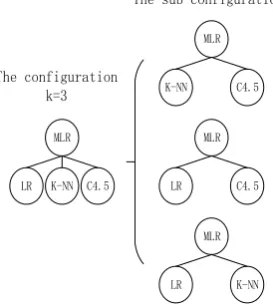
Not only the fitness but also the ensemble size are considered to discriminate the unnecessary individuals. Considering a configuration c with k (≥2) base classifiers, we can obtain k configurations by removing one of the base classifiers from it and these k configurations are called c’s

sub-configurations, as the example shown in Figure 3. Once find a sub-configuration sc whose fitness is equal to or higher than c’s, c will be regarded as the unnecessary configuration and the individual will be discriminated as the unnecessary individual because compared to c, sc seems to have an equivalent and even higher performance with a smaller size.

Figure 3. The example of the configuration and its sub-configurations, k=3. The configuration consists of MLR as the meta classifier, Logistic Regression, K-NN and C4.5 decision tree as the base classifiers.

The tabu table and the generated set are introduced to reduce the reproduction of unnecessary individuals (Figure 2). The generated set stores all of the individuals generated in the GA process. When a new population is generated, the generated set will be updated and the tabu table will be updated from the generated set. In the next generation, if an individual in the tabu table is generated

New Population

Population

Fitness Evaluation

End?

Elitism/Culling

Crossover

Mutation No evaluating

Generated Set

Tabu

Local Best Config

Yes

Check

GA process

Update

Update

MLR

K-NN C4.5

MLR

LR K-NN C4.5

MLR

LR C4.5

MLR

LR K-NN

The configuration k=3

again in the crossover and mutation operation, the operation will be redone until the max trial value is reached.

Figure 4. The algorithm of AGA-E.

Figure 5. The algorithm of GAProcessOn.

Phases of AGA-Ensemble

search process. Then, the evaluating part is used to calculate the fitness. In order to save the training time, the pool of b candidate base classifiers is generated in this phase[14]. In GA Search phase (line 7-10), m GA search processes are running to select the LBCs. The pseudocode of GAProcessOn is shown in Figure 5. In the last phase (line 11-14), the final configuration is selected and then the corresponding stacking ensemble classifier is trained on the whole training set as the output of the approach.

Experiments and Results

Experimental Setups

To investigate the performance of AGA-E, the preliminary experiments are conducted in WEKA[17]. This environment includes some well-known ensemble method and all the candidate algorithms for meta and base classifiers in the experiments.

13 benchmarked classification datasets in different domains from the UCI machine learning repository[18] are used. Some basic information of these datasets is listed in Table 1. The same in [14], all the datasets are used without any preprocessing or feature selection.

Table 1. The description of datasets.

Dataset Attributes Instances Classes

Iris 4 150 3

Hepatitis 19 155 2

Wine 13 178 3

Heart-statlog 13 270 2

Sonar 61 208 2

Ionosphere 34 351 2

Glass 9 214 6

Breast-w 9 699 2

Balance 4 625 3

Credit-a 14 690 2

Diabetes 8 768 2

Credit-g 21 1000 2

Vehicle 19 846 4

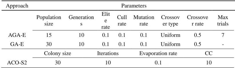
Table 2. The parameters of AGA-E, GA-E and ACO-S2.

Approach Parameters

Population size Generation s Elit e rate Cull rate Mutation rate Crossov er type Crossove r rate Max trials

AGA-E 15 10 0.1 0.1 0.1 Uniform 0.5 7

GA-E 30 10 0.1 0.1 0.1 Uniform 0.5 -

Colony size Iterations Evaporation rate CC

ACO-S2 30 10 0.1 10

10 different learning algorithms in WEKA are used to generate the candidate base classifiers in AGA-E. They are J48, Decision Stump, PART, Naïve Bayes, IB1, IBk, KStar, Logistic Regression, OneR and ZeroR, which are used in [14]. Except ZeroR, they and MRMT are used to generate the candidate meta classifier, which makes sure the intersection of the search spaces of AGA-E and GA-E.

And AGA-E is compared to the following 7 ensemble approaches. The parameters of AGA-E, GA-E and ACO-S2 in the experiments are shown in Table 2.

• AdaBoost using C4.5 decision trees as base classifiers.

• Bagging using C4.5 decision trees as base classifiers.

• StackingC using Naïve Bayes, IBk and C4.5 decision tree as the base classifiers and MRMT as the meta classifier.

• GA-E using the same candidate base classifiers as AGA-E.

• ACO-S2 using the same base and meta candidate classifiers as AGA-E.

Evaluation

To make the experiment results more robust, the 10-fold cross validation is adopted to calculate the average accuracy of each approach on each dataset. Then AGA-E’s relative improvement, RAI[14], with other approaches are calculated. In addition, the paired T-test, Sign test[19], non-parametric Friedman test[20] and the Holm’s procedure[21] are conducted to illustrate the statistical significance between AGA-E and other approaches. Besides to show the utility of the tabu strategy, the average rates of the re-operations of AGA-E are calculated.

Results and Analysis

The results of the average accuracies of the approaches and the results of the paired T-test on 13 datasets are shown in Table 3. The maximum on each dataset are marked in bold and the significant results are denoted by superscript.

Table 3. The accuracies of the approaches.

Dataset AdaBoost Bagging Random

Forest StackingC GA-E ACO-S2 AGA-E

Iris 94.00 93.33 94.67 94.67 95.33 92.00 96.00

Hepatitis 82.67 80.58 83.13 79.54 83.79 83.42 81.25

Wine 95.85 96.47 98.24 96.47 96.99 96.47 98.24

Heart-statlog 78.15 80.00 82.96 84.44 82.59 84.44 84.82

Sonar 79.26c 75.02b 81.19 81.76 83.19 84.17 86.05

Ionosphere 93.18 91.45 93.17 88.58 92.02 93.17 91.16

Glass 73.40 73.85 76.15 71.93c 74.37 76.26 77.53

Breast-w 96.28 95.99 96.14 96.71 95.99 96.28 96.85

Balance 78.40a 84.16a 81.46a 90.40a 94.26 93.91 94.57

Credit-a 83.19 86.38 86.67 85.80 85.36 85.65 85.65

Diabetes 71.10b 74.34 75.51 76.30 76.68 75.92 75.64

Credit-g 71.10b 75.20 74.70 75.50 76.30 75.70 77.10

Vehicle 75.29a 73.17a 75.65a 74.35a 80.97 80.51 81.33

w/t/l _{11/ 0/ 2 11/ 0/ 2 9/ 1/ 3 11/ 0/ 2 10/ 0/ 3 9/ 1/ 3 -}

a _{worse than AGA-E at the 1% significant level in the paired T-test.} b _{worse than AGA-E at the 5% significant level in the paired T-test.} c _{worse than AGA-E at the 10% significant level in the paired T-test.}

AGA-E achieves the maximum on 9 datasets while Random Forest, GA-E and AdaBoost achieve 2, 2 and 1 respectively and the rest of approaches have no maximum on any dataset. However, in the result of T-test, AGA-E significantly outperforms AdaBoost, Bagging, Random Forest and StackingC on some of the 13 datasets and is not significantly better than GA-E and ACO-S2 on any single dataset. Moreover, AGA-E is not significantly worse than these 6 approaches on any dataset.

The counts of wins, ties and losses of AGA-E to other approaches over all datasets are also shown in the last row of Table 3. The sign test makes use of the w/t/l values to reveal the significant differences over multiple datasets[19]. The results indicate that AGA-E outperforms AdaBoost, Bagging, StackingC and GA-E at the 5% significant level. But when compared to Random Forest and ACO-S2, AGA-E holds 9/1/3 on the w/t/l, which means the advantage of AGA-E is not significant but is near the 10% significant level.

RAI measures the AGA-E’s relative improvement with other approaches across multiple datasets. It is calculated by Eq. 1.

𝑅𝐴𝐼(𝑥) = ∑ 𝐴𝑐𝑐(𝑖,𝐴𝐺𝐴)−𝐴𝑐𝑐(𝑖,𝑥)

𝐴𝑐𝑐(𝑖,𝑥)

where 𝐴𝑐𝑐_{(𝑖,𝐴𝐺𝐴)} and 𝐴𝑐𝑐_(𝑖,𝑥) refer to the average accuracy of AGA-E and approach x on dataset i

respectively. In Table 4, AGA-E gets a relative improvement of 70.49% with AdaBoost, 58.74% with Bagging, 37.00% with StackingC, 33.58% with Random Forest, 10.10% with GA-E and 9.57% with ACO-S2.

Table 4. The RAI results.

AdaBoost Bagging Random Forest StackingC GA-E ACO-S2 AGA-E RAI

(%) 70.49 58.74 33.58 37.00 10.10 9.57 -

In the Friedman test and the Holm’s procedure, we focus on comparing the performances of GA-E, ACO-S2 and AGA-E over multiple datasets[22]. The p-value obtained from the Friedman test is 8.29%(<10%), which indicates that the performances of these 3 approaches are significantly different at the 10% level. In Table 5, the average ranks and the adjusted p-values obtained from the Holm’s procedure indicate that AGA-E has a better performance than ACO-S2 and GA-E at the 10% significant level.

Table 5. The results of the Holm’s procedure.

ACO-S2 GA-E AGA-E

Average rank 2.269 2.231 1.500

Adjusted p-value

(%) 9.97 6.24 -

According to the results of various tests, it is summarized that although having a slightly advantage on the single dataset, AGA-E significantly outperforms other approaches over multiple datasets.

The re-operation rate (ROR) of AGA-E is calculated by Eq. 2.

𝑅𝑂𝑅(𝑖) = 𝑅𝑒𝑂𝑝(𝑖)

𝑂𝑝(𝑖) . (2) The 𝑅𝑒𝑂𝑝(𝑖) and 𝑂𝑝(𝑖) refer to the number of the re-operations and the number of the operations on

the dataset i respectively. When multiple re-operations are caused by an operation, they count only once. The 𝑅𝑂𝑅(𝑖) represents the proportion of the unnecessary reproduction in the GA search and indicates the frequency of using the tabu strategy of AGA-E on dataset i. In Figure 6, the ROR ranges from 13% to 19%, which means that there are a quite number of the unnecessary reproductions in the GA search. On one hand, it is worthy of the tabu strategy, on the other hand it confirms that GA search in the configuration selection is promising because of the ROR being not too high.

Figure 6. The results of ROR.

Conclusion and Future Work

superior to GA-E over multiple datasets but is slightly better than GA-E on the single dataset and indicates the value of the tabu strategy introduced. Therefore, the new approach has a higher adaptability and a better performance.

In future work, not only the benchmarked UCI datasets, the real-life application datasets will be used to test the performance of AGA-E.

Acknowledgement

This research was financially supported by the National Natural Science Foundation of China (61402514).

References

[1] D.A. Morales, E. Bengoetxea, P. Larrañaga, Gaussian-stacking multiclassifiers for human embryo selection, Data Mining & Medical Knowledge Management Cases & Applications. (2009).

[2] E. Hadavandi, Effective Intrusion Detection with a Neural Network Ensemble Using Fuzzy Clustering and Stacking Combination Method, (2015).

[3] L. Kai, T. Plötz, G.A. Fink, Stacking for Ensembles of Local Experts in Metabonomic Applications, in: International Workshop on Multiple Classifier Systems, 2009: pp. 498–508.

[4] A. Venugopal, Nisha, A New Personalized Product Recommender System Using Stacking and Memory Based Collaborative Algorithm, (2015).

[5] S. Karaman, L. Seidenari, A.D. Bagdanov, L1-regularized Logistic Regression Stacking and Transductive CRF Smoothing for Action Recognition in Video, (2013).

[6] J. Sill, G. Takacs, L. Mackey, D. Lin, Feature-Weighted Linear Stacking, Computer Science. (2009).

[7] M.T. Kai, I.H. Witten, I.H, Issues in stacked generalization, (1999).

[8] L. Todorovski, S. Džeroski, Combining Multiple Models with Meta Decision Trees, in: Principles of Data Mining and Knowledge Discovery, European Conference, Pkdd 2000, Lyon, France, September 13-16, 2000, Proceedings, 2000: pp. 54–64.

[9] A.K. Seewald, How to Make Stacking Better and Faster While Also Taking Care of an Unknown Weakness, in: Nineteenth International Conference on Machine Learning, 2002: pp. 554–561.

[10] S. Dzeroski, B. Zenko, Is Combining Classifiers Better than Selecting the Best One, in: Nineteenth International Conference on Machine Learning, 2002: pp. 255–273.

[11] D.E. Goldberg, J.H. Holland, Genetic algorithms and machine learning, Machine Learning. 3 (1988) 95–99.

[12] M. Dorigo, Optimization, Learning and Natural Algorithms, Thesis Politecnico Di Milano Italy. (1992).

[13] F.J. Ordóñez, A. Ledezma, A. Sanchís, Genetic Approach for Optimizing Ensembles of Classifiers., in: International Florida Artificial Intelligence Research Society Conference, May 15-17, 2008, Coconut Grove, Florida, Usa, 2008: pp. 89–94.

[14] Y.J. Chen, M.L. Wong, H. Li, Applying Ant Colony Optimization to configuring stacking ensembles for data mining, Expert Systems with Applications. 41 (2014) 2688–2702.

[15] D.H. Wolpert, Stacked Generalization, Neural Networks. 5 (1992) 241–259.

[17] I.H. Witten, M. Hall, E. Frank, G. Holmes, B. Pfahringer, P. Reutemann, The weka data mining software: an update, Acm Sigkdd Explorations Newsletter. 11 (2009) 10–18.

[18] M. Lichman, UCI Machine Learning Repository, University of California, Irvine, School of Information and Computer Sciences, 2013. http://archive.ics.uci.edu/ml.

[19] M.S. Nash, Handbook of Parametric and Nonparametric Statistical Procedures, American Statistician. 43 (1998) 382–382.

[20] M. Friedman, The Use of Ranks to Avoid the Assumption of Normality Implicit in the Analysis of Variance, Journal of the American Statistical Association. 32 (2012) 675–701.

[21] S. Holm, A simple sequentially rejective multiple test procedure, Scandinavian Journal of Statistics. 6 (1979) 65–70.