A Novel Adaptive Chaotic Bacterial Foraging Optimization Algorithm

2016 International Conference on Computational Modeling, Simulation and Applied Mathematics (CMSAM 2016) ISBN: 978-1-60595-385-4

A Novel Adaptive Chaotic Bacterial Foraging Optimization Algorithm

Yuan-tao ZHANG*, Wei ZHOU and Jun YI

College of Electrical and Information Engineering, Chongqing University of Science and Technology, Chongqing 401331, China

*Corresponding author

Keywords: Bacterial foraging optimization, Chaotic map, Adaptive chemotaxis step.

Abstract. In this paper, an adaptive chaotic bacterial foraging optimization (ACBFO) is presented. The improved bacterial foraging algorithm contains two new features, adaptive chemotaxis step setting and chaotic perturbation operation in each chemotactic event. The adaptive chemotaxis step setting enables fast convergence speed and good convergence accuracy of the algorithm, and the bacteria chaotic perturbation operation further allows the search to escape from local optima and achieve better convergence accuracy. With five benchmark functions, ACBFO is proved to have a better performance than the original bacterial foraging optimization (BFO) and BFO with linear deceasing chemotaxis step (BFO-LDC).

Introduction

Bacterial foraging optimization (BFO) is a new bionic evolution algorithm presented by Passino in the early 2002[1]. It simulates the foraging behavior of human Escherichia coli in order to reach a nutrient-rich place. BFO searches automatically for the optimum solution in the search space by means of chemotaxis, swarming, reproduction, elimination and dispersal. Recently, BFO algorithm has rapidly become popular and has been applied to solve various optimization problems. BFO owns the characteristics of swarm intelligence parallel search and sophisticated search ability. But in the same time, the drawback of consistent chemotaxis step makes BFO unable to achieve exploration and exploitation tradeoff, which results in easily trapping into local optima and slow convergence speed. Therefore, many researchers have made improvements to BFO[2,3]. As a kind of evolution phenomenon of nonlinear system, chaos is a stochastic state in the deterministic system, which owns the characteristics of ergodicity, stochasticity and regularity. Owing to chaos optimization method has the advantages of global asymptotic convergence, easy to jump out of local minima and fast convergence speed, nowadays it is widely used in various kinds of optimization algorithms to improve their optimization performances [4,5].

In this paper, the authors propose an adaptive chaotic bacterial foraging optimization algorithm inspired by linear deceasing chemotaxis step and chaos theory in this paper. Firstly, an idea of adaptive exponential deceasing chemotaxis step is presented, in which the natural exponential function variable is a function about the iterations and nutritive ratio between the current bacterium position and the best bacterium position in each iteration. Secondly, when each bacterium reaches a new position through swim behavior, chaotic perturbation is applied to avoid entrapping into local optima. In order to demonstrate the performance of the proposed algorithm, ACBFO is applied into five benchmark functions and the experiment results demonstrate ACBFO is superior to the original BFO and BFO-LDC algorithms.

Adaptive Chaotic Bacterial Foraging Optimization

Adaptive Chemotaxis Step Setting

of the search. When C is too large, the bacteria will fail to locate the global optimum by swimming without stop. While C is too small, it will take a long time for the bacteria to find the global optimum. Therefore, an expected result with faster searching time and global optimal orientation can be obtained by choosing intermediate C. Niu, et al [2] proposed a linearly decreasing chemotaxis step over iterations, though it shows some improvement in convergence speed and accuracy, it still easily entraps into local optima for all bacteria using same C in each iteration, which inspired by the idea of linearly decreasing chemotaxis step, the authors present an adaptive chemotaxis step strategy as following:

( , , , ) last/ best( , , )

f i j k l = ×η J J j k l (1)

( , , , )/

max max min

( , , , ) ( ) f i j k l j

C i j k l =C − C −C ×e− (2)

where Jlast=J i j k l( , , , ) represents the ith bacterium best cost function value at jth chemotactic and kth

reproductive and lth elimination and dispersal event. Jbest( , , )j k l represents the best cost function value

of population. C i j k l( , , , )is the chemotaxis step size and η is a constant named restriction factor. The smaller value of k will make C i j k l( , , , )decreases rapidly and the larger value of k will make C i j k l( , , , )

change slowly. Considering ( , , , )/

0 f i j k l j 1 e−

< < , thus C i j k l( , , , ) [∈Cmin,Cmax], as is shown in Figure 1. Because

( , , , ) /

f i j k l jwill generally decrease with the increasing of iteration number j, therefore, the general

trend of C i j k l( , , , ) is decreasing with the increasing of iteration number j, which results in fast

convergence of BFO. This is some like the ideal of linearly decreasing chemotaxis step, but the difference of our strategy lies in that f i j k l( , , , )can adaptively change in terms of the ratio of the cost

function value of ith bacterium to the best cost function value of population. Smaller f i j k l( , , , ) means

the ith bacterium is close to the optimum solution of population, which leads to the decreasing of

( , , , )

C i j k l to search for better solutions. And biggerf i j k l( , , , ) means the ith bacterium is far from the

optimum solution of population, which leads to the increasing of C i j k l( , , , )to avoid early convergence.

In one word, the adaptive chemotaxis step the authors proposed can dynamically adjust the chemotaxis step in terms of the cost function value of each bacterium and iteration numberj, in

which the main advantage is fast convergence speed and good convergence accuracy.

0 1 2 3 4 5 6 7 8 9 10

0 0.02 0.04 0.06 0.08 0.1 0.12 0.14 0.16 0.18 0.2

f(i,j,k,l)/j

C

h

e

m

o

ta

x

is

s

te

p

C

(i

,j

,k

,l

)

Figure 1. Adaptive chemotaxis step (e.g.Cmin=0.001,Cmax=0.2).

Chaotic Perturbation Operation

(t 1) ( )t (1 ( )t )

U ₊ = µ×U × −U ₍₃₎

where U( )t represents the tth chaotic number and t is the iteration number.µ is the control parameter controlling the behavior of U( )t (as t goes to infinity). The behavior of the logistic map for various values of the parameter µ _{is shown in Figure 2 For low values of} µ ₍µ _{< 3),} U _{eventually converges}

to a single number. Whenµ =3_, U _{oscillates between two values. This characteristic change in}

behavior is called bifurcation. Forµ >3_, U _{goes through further bifurcations, eventually resulting in}

chaotic behavior. Obviously, when µ =4_{, the chaotic sequence value} U_{is bounded within}(0,1)_under

the conditions that the initial U( )t ∈(0,1) and that U( )t∉{0, 0.25, 0.5, 0.75,1}. Figure 3 shows the chaotic U value of a logistic map for 100 iterations where U(0)=0.005.

2.6 2.8 3 3.2 3.4 3.6 3.8 4

0 0.2 0.4 0.6 0.8 1

Control parameter µ

C

h

a

o

ti

c

U

v

a

lu

e

Figure 2. Bifurcation diagram of logistic map.

Figure 3. Dynamics of logistic map.

Specifically, according to the study conducted by Passino [1], the chemotactic event is generally the key event affecting the convergence performance of BFO. Therefore, this paper incorporates chaotic mapping with ergodic, stochastic, and regular properties in each chemotactic event of the bacterium to improve the global convergence. The use of chaotic sequence in BFO can facilitate escaping from local optima and exploring for better solutions. In this study, the authors combine the logistic map with bacterial foraging optimization in chemotactic event named chaotic perturbation.

In the process of chaotic perturbation operation for a p-dimensional optimization problem, according to Eq.(1), firstly, the N-dimensional initial vector Z0 bounded within(0,1)is generated

randomly as Z0=(Z01,Z02,Z0p). Furthermore, Z0 is not equal to {0, 0.25, 0.5, 0.75,1}and µ equal to 4.Then in

each swim behavior of chemotactic event, Z1=(Z11,Z12,Z1p) can be obtained by means of

1i 4 0i (1 0i), 1, 2,

Z = ×Z × −Z i= p (4)

And then each components of Z1 is carried to the chaotic perturbation range (−β β, ) . The

perturbation value ∆X= ∆( X1,∆X2,∆Xp)can be achieved computing

1

2 , 1, 2,

i i

X β β Z i p

∆ = − + × = (5)

After this step, one thing to be noted is thatZ1=Z0, which could help Z1traverse the whole space

within(−β β, )_{. Finally, the new bacterium position is the sum of the current position without chaotic}

perturbation and ∆X. Comparing the cost function value of the new position with that of the current position without chaotic perturbation will lead to the choice of the better position with lower cost function value.

Pseudo-code of ACBFO

According to the discussion above, the adaptive chaotic bacterial foraging algorithm the authors called ACBFO has two new features, adaptive chemotaxis step setting and chaotic perturbation operation. The adaptive chemotaxis step setting enables fast convergence speed and good convergence accuracy of the algorithm, and the bacteria chaotic perturbation operation further allows the search to escape from local optima and explore for better solutions.

During the process of solving actual optimization problems, it is usually unnecessary to consider the cell-to-cell signaling attractant-repellentJcc between bacteria. Let i be the index for the bacterium in population. Let j,k,l be the indexes for the chemotactic, reproductive, elimination and dispersal events respectively. Let _{P j k l}( , , )₌{_θi( , , ) |_{j k l i=}1, 2, ,_S}

represents the bacterium position in population and

( , , , )

J i j k l _{represents the cost function value .Let} t represents the total iteration numbers. Also let

p_{: Dimension of the search space} S_{: Total number of bacteria in the population}

c

N _{: Number of chemotactic events} Ns: Swim length

re

N _{:Number of reproductive events} Sr: Number of bacteria reproductions per generation

ed

N _{: Number of elimination and dispersal events} Ped: Elimination and dispersal probability

( , , , )

C i j k l _{: Cheomotaxis step size} η_{: Restriction factor of adaptive chemotaxis step} β_{: Chaotic perturbation range parameter} Z( )t : Chaotic vector

The pseudo-code of ACBFO process for actual optimization problems is shown below.

Table 1. Pseudo-code of ACBFO.

[Step1] Initialize parametersp_,S,

r

S ，Nc,Ns,Nre,Ned,Ped,Cmax,Cmin,η,β, randomly generate ( 1, 2, , )

i

i S

θ = in the search

space and initial chaotic vector (0)

p

Z ∈R _within (0,1) _{but not equals to} {0, 0.25, 0.5, 0.75,1}_.

[Step2] Elimination and dispersal loop: l= +l 1

[Step3] Reproduction loop: k= +k 1

[Step4] Chemotaxis loop: j= +j 1

[a] Firstly for i=1, 2,S compute the cost function value J i j k l( , , , ), sort J i j k l( , , , )to find the lowest cost Jbest( , , )j k l . [b] Then for bacterium i(firstly let i=1), compute cost function valueJ i j k l( , , , ).

[c] Let Jlast=J i j k l( , , , )to save this value since we may find a better cost via a run.

[d] Compute the adaptive chemotaxis step C i j k l( , , , ) ( , , , ) last/ best( , , )

f i j k l = ×η J J j k l _, ( , , , )/ max max min

( , , , ) ( ) f i j k l j

C i j k l C C C e−

= − − ×

[e] Tumble: generate a random vector ( ) p

i R

∆ ∈ in the interval [ 1,1]− [f] Move: Let ( 1, , ) ( , , ) ( , , , ) ( )

( ) ( )

i i

T

i j k l j k l C i j k l

i i

θ + =θ + ∆

∆ ∆ . This results in a step of size C i j k l( , , , ) in the direction of the tumble for bacterium i_.

[g] Compute J i j( , +1, , )k l _.

[h] Swim

(1) Let m=0(counter for swim length)

(2) While m<Ns(if have not climbed down too long) Let m=m+1.

IfJ i j( , +1, , )k l <Jlast,let Jlast=J i j( , +1, , )k l and let

( ) ( 1, , ) ( , , ) ( , , , )

( ) ( )

i i

T

i j k l j k l C i j k l

i i

θ + =θ + ∆

∆ ∆

Then use this i( 1, , ) j k l

θ + to compute the newJ i j( , +1, , )k l _{as we did in [h], and add chaotic perturbation as follows:} Generate chaotic vectorZ1=(Z11,Z12,Z1p)where

1i 4 0i (1 0i), 1, 2,

Z = ×Z × −Z i= p.This is generated according to logistic map defined in Eq. (3) Each components of Z1 is carried to the chaotic perturbation range(−β β, ). The perturbation value

1 2

( , , p) X X X X

∆ = ∆ ∆ ∆ can be achieved computing ∆Xi= − +β 2β×Z i1i, =1, 2,p

Use i( 1, , ) j k l

If Jcp( ,i j+1, , )k l <J i j( , +1, , )k l , let ( 1, , ) ( 1, , )

i i

i

j k l j k l X

θ + =θ + + ∆ .

Z0=Z1. This can help Z1traverse the whole space bounded within(0,1), in other words, ∆X can traverse

the whole perturbation space bounded within (−β β, ).

Else ,let m=Ns.This is the end of the while statement. [i] Go to [b] to process the next bacterium (i+1) _if i≠S.

[Step5] If j<Nc,go to step 4 to continue chemotaxis since the life of the bacteria is not over.

[Step6] Reproduction:

[a] For i=1, 2,S, compute the health of bacterium i as follow:

1 1 ( , , , ) c N i health j

J J i j k l

+

=

=∑ .This is a measure of how many nutrient it got over its lifetime and how successful it was at avoiding noxious substances.

[b] Sort bacteria and chemotaxis step C i j k l( , , , )_{in order of ascending cost} Jhealth(higher cost means lower health). [c] The Srbacteria with the highest Jhealth values die and the remaining Sr bacteria with the best values split into two

copies which are placed in the same lactation as their parent.

[Step7] If k<Nre, go to step 3 and start the next generation of chemotactic loop.

[Step8] Elimination and dispersal: For i=1, 2,S, eliminate and disperse bacterium i with probability Ped.If a bacterium is eliminated, simply disperse another one to a random position on the optimization domain to keep population constant. If

ed

l<N _{,go to step 2,otherwise end.}

Simulation Research

To evaluate the performance of ACBFO algorithm the authors proposed, standard BFO[6] and BFO-LDC[2] are compared with ACBFO in terms of solution quality and convergence speed. The test suite includes five well-known benchmark functions, which can be classified into uni-modal functions (f f1, 2) and multi-modal functions (f3,f4,f5).The optimization goal for each function is to find

the global minimum. The functions are listed as following:

Sphere function 2

1 1 ( ) n i i

f x x

=

=

∑

Rosenbrock function

1

2 2 2

2 1

1

( ) (100( ) ( 1) ) n

i i i

i

f x x x x

− + =

=

∑

Generalized Rastrigin function 2 3

1

( ) ( 1 0 c o s ( 2 ) 1 0 )

n

i i

i

f x x π x

=

= ∑ − + _{, where} −10≤x_i≤10 (8)

Griewank function 2

4

1 1

1

( ) c o s 1

4 0 0 0

n n i i i i x

f x x

i

= =

 

= −  +

 

∑ ∏ , where −600≤xi≤600 (9)

Ackley function 2

5

1 1

1 1

( ) 2 0 ex p 0 .2 ex p co s( 2 ) 2 0

n n

i i

i i

f x x x e

n = n = π

   

= − _− _−  + +

 

 ∑  ∑ , where −3 0≤ xi≤3 0 (10)

Table 2. Parameter settings for benchmark functions. Function Dim Minimum

value

Iterations Search range Asymmetrical initialization range

1

f 15 0 10000 15

[ 100,100]− 15

[50,100]

2

f 15 0 10000 15

[ 100,100]− 15

[15, 30]

3

f 15 0 10000 _{[ 10,10]−} 15 _{[2.56, 5.12]}15

4

f 15 0 10000 15

[ 600, 600]− 15

[300, 600]

5

f 15 0 10000 15

[ 30, 30]− 15

[15, 30]

Table 3. Parameter settings of ACBFO.

f p S N_c Ns Nre Sr Ned Ped Cmax Cmin k β

1

f 15 20 1000 4 5 10 2 0.25 0.2 0.001 0.1 0.1

2

f 15 20 1000 4 5 10 2 0.25 0.2 0.001 0.1 0.1

3

f 15 20 1000 4 5 10 2 0.25 0.2 0.001 1 10

4

f 15 20 1000 4 5 10 2 0.25 1 0.001 1 0.5

5

f 15 20 1000 4 5 10 2 0.25 0.6 0.001 3 10

Table 3 lists the parameters values in ACBFO for five benchmark functions. The corresponding parameters values in BFO-LDC and standard BFO are the same as that in ACBFO. In BFO-LDC, the range of linear decreasing chemotaxis step [Cmin,Cmax] is consistent with that in ACBFO to make the

comparison fair. In standard BFO, the fixed chemotaxis step Cis respectively 0.1 (f1,f2,f3), 0.5

(f4)and 0.3(f5). The results reported in this section are averaged over 20 times experiments.

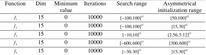
Table 4. Fitness value for Sphere function.

Algorithms Best Worst Mean Std

BFO 0.0722 0.1421 0.1099 0.0241

BFO-LDC 0.0016 0.0054 0.0033 0.0012

ACBFO 1.1159e-005 1.5797e-005 1.3534e-005 1.7303e-006

Table 5. Fitness value for Rosenbrock function.

Algorithms Best Worst Mean Std

BFO 21.2077 125.7414 51.4991 39.1549

BFO-LDC 9.9494 35.2055 18.3289 9.8620

ACBFO 5.4607 16.4185 10.5280 3.1144

Table 6. Fitness value for Generalized Rastrigin function.

Algorithms Best Worst Mean Std

BFO 45.4104 61.4364 51.4160 4.7869

BFO-LDC 24.0425 38.2708 29.9072 4.1886

ACBFO 10.9733 18.9634 15.5849 2.6082

Table 7. Fitness value for Griewank function.

Algorithms Best Worst Mean Std

BFO 0.2089 0.3276 0.2673 0.0368

BFO-LDC 0.0188 0.0447 0.0266 0.0084

ACBFO 5.5735e-006 0.0369 0.0096 0.0113

Table 8. Fitness value for Ackley function.

Algorithms Best Worst Mean Std

BFO 2.8065 17.6162 9.0029 5.9573

BFO-LDC 1.5606 17.0030 6.1943 5.7138

ACBFO 0.0318 0.9419 0.1382 0.2826

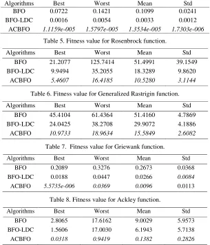
Figures 4-8. shows the comparison of the convergence speed and accuracy of basic BFO, BFO-LDC and ACBFO during 10000 iterations for five benchmark functions respectively. From these Figures, we can find that the performance of ACBFO is significantly superior to basic BFO and BFO-LDC for five classic test functions not only in convergence speed but also in convergence accuracy, especially to some complex optimization problemsf4and f5. The stimulation results are also

obtains the best results with the comparison of BFO and BFO-LDC except a little bigger standard deviation value than BFO-LDC for Griewank function.

0 1000 2000 3000 4000 5000 6000 7000 8000 9000 10000 -15 -10 -5 0 5 10 15 Iteration F it n e s s ( lo g ) BFO BFO-LDC ACBFO

Figure 4. Convergence curve for Sphere function. Figure 5. Convergence curve for Rosenbrock function.

0 1000 2000 3000 4000 5000 6000 7000 8000 9000 10000 2 2.5 3 3.5 4 4.5 5 5.5 6 Iteration F it n e s s ( lo g ) BFO BFO-LDC ACBFO

0 1000 2000 3000 4000 5000 6000 7000 8000 9000 10000 -8 -6 -4 -2 0 2 4 6 8 Iteration F it n e s s ( lo g ) BFO BFO-LDC ACBFO

Figure 6. Convergence curve for Generalized Rastrigin function. Figure 7. Convergence curve for Griewank function.

0 1000 2000 3000 4000 5000 6000 7000 8000 9000 10000

-3 -2 -1 0 1 2 3 4 Iteration F it n e s s ( lo g ) BFO BFO-LDC ACBFO

Figure 8. Convergence curve for Ackley function.

Conclusions

References

[1] K.M. Passino, Biomimicry of bacterial foraging for distributed optimization and control, IEEE Control Systems Magazine 22(3) (2002) 52-67.

[2] B. Niu, Y. Fan, H. Xiao, X. Bing, Bacterial foraging based approaches to portfolio optimization with liquidity risk, Neruocomputing 98 (2012) 90-100.

[3] M.S. Li, T.Y. Ji, W.J. Tang, Q.H. Wu, J.R. Saunders, Bacterial foraging algorithm with varying population, Biosystems 100(3)(2010) 185-197.

[4] A.H. Abdullah, R. Enayatifar, M. Lee, A hybrid genetic algorithm and chaotic function model for image encryption, AEU-International Journal of Electronics and Communications 66(10) (2012) 806-816.

[5] S.S. Chen, Chaotic Simulated Annealing by a Neural Network with a Variable Delay: Design and Application, IEEE Transactions on Neural Networks 22(10) (2011) 1557-1565.