Twin constrained Hamiltonian paths on threshold graphs: an approach to the minimum score separation problem

(1)

The London School of Economics and Political Science

Twin-Constrained Hamiltonian Paths

on Threshold Graphs

- an Approach to the Minimum Score Separation Problem

Kai Helge Becker

(2)

Declaration

I certify that the thesis I have presented for examination for the PhD degree of the London School of Economics and Political Science is solely my own work other than where I have clearly indicated that it is the work of others (in which case the extent of any work carried out jointly by me and any other person is clearly identi…ed in it).

The copyright of this thesis rests with the author and no quotation from it or information derived from it may be published without the author’s written consent. This thesis may not be reproduced without the prior written consent of the author.

(3)

Abstract

The Minimum Score Separation Problem (MSSP) is a combinatorial problem that has been introduced in JORS 55 as an open problem in the paper industry arising in conjunction with the cutting-stock problem. During the process of producing boxes, ‡at papers are prepared for folding by being scored with knives. The problem is to determine if and how a given production pattern of boxes can be arranged such that a certain minimum distance between the knives can be kept. While it was originally suggested to analyse the MSSP as a speci…c variant of a Generalized Travelling Salesman Problem, the thesis introduces the concept of constrained Hamiltonian cycles and models the MSSP as the problem of …nding a twin-constrained Hamiltonian path on a threshold graph (threshold graphs are a speci…c type of interval graphs).

For a given undirected graph G(N,E) with an even node set N and edge set E, and a bijective function b on N that assigns to every node i in N a "twin node" b(i)₆=i, we de…ne a new graph G’(N,E’) by adding the edges {i,b(i)} to E. The graph G is said to have a twin-constrained Hamiltonian path with respect to b if there exists a Hamiltonian path on G’ in which every node has its twin node as its predecessor (or successor).

(4)

Acknowledgements

First of all, I am very much indebted to my supervisor Professor Gautam Appa, who has greatly inspired my research, and my life beyond - in fact, to far greater an extent than he is probably aware of. Also, I am very grateful for his permanent support and his understanding of what drives me academically.

Also, I would like to thank the sta¤ members (and later colleagues) at the Operational Research Group at LSE, who all contribute to making the group (and LSE in general) an inclusive and stimulating environment for research that brings to life the spirit that characterises a true university. In particular I am thankful to Dr Barbara Fasolo, Dr Gilberto Montibeller, Dr Alec Morton, Dr Katerina Papadaki, Professor Larry Phillips, Dr Alan Pryor and Professor Paul Williams for interesting insights and both helpful comments and advice on various academic matters in the past years. Moreover, the working environment of the Operational Research Group would have been much less productive and pleasant a place, if the group were not run as excellently on the administrative side as it actually is. I am very grateful to Brenda Mowlam, Jenny Robinson, Richard Szadura and Lucy Underhill for their great support, helpful advice and amazing kindness over all the years, from my …rst steps at LSE to my time as a member of sta¤.

I would also like to thank all my fellow PhD students at LSE, especially Dr Nikos Argyris, Florian Gebreiter, Nayat Horozoglu, Attila Marton and Dr Kostas Papalamprou, who all have, in one way or the other, contributed to making LSE my home, on both the academic and the personal level. I am particularly thankful to Dr Nikos Argyris, with whom I undertook the very …rst steps in analysing the problem that would later become the topic of this thesis; unfortu-nately, he had to focus his attention on his own thesis after a short time. Also, I am thankful to Dr Kostas Papalamprou for a great introduction into the topic of total unimodularity, and I would like to thank my fellow PhD students for their friendship and great sense of community. Moreover, I am grateful to Frits Spieksma from the Univeristy of Leuven for his interest in the theoretical aspects of this thesis and several insightful discussions.

Many thanks are also due to British Petroleum who generously funded most of the research undertaken in this thesis.

(5)

List of Figures

1 Feasible alignment of boxes I . . . 11

2 Feasible alignment of boxes II . . . 12

3 The MSSP as a Traveling Politician Problem . . . 16

4 The MSSP as a twin-constrained Hamiltonian path problem . . . 21

5 Examples of threshold graphs . . . 39

6 Examples of non-threshold graphs . . . 40

7 Degree partition of a threshold graph . . . 42

8 Structures of G and G’. . . 54

9 The twin-induced structure of a matching . . . 77

10 The case_jM_j=n . . . 80

11 The case_jM_j=n-1 . . . 81

12 Matching, twin-node function and (in)feasibility . . . 82

13 Constructing a feasible solution to the MSSP . . . 83

14 Types of structure-preserving solutions . . . 84

15 Irreducible path-splitting solutions . . . 89

16 Solutions with a cycle-split . . . 96

17 A-matrix of the modi…ed ‡ow problem . . . 114

18 Constructing a solution by means of alternatingT-cycles . . . 122

List of Tables

1 MSSPH, uniform distribution I . . . 146

2 MSSPH, uniform distribution II . . . 147

3 MSSPH, uniform distribution III . . . 148

4 MSSPH, triangular distribution I . . . 149

5 MSSPH, triangular distribution II . . . 150

6 TGHRA, uniform distribution I . . . 151

7 TGHRA, uniform distribution II . . . 151

8 TGHRA, uniform distribution III . . . 152

9 TGHRA, triangular distribution I . . . 152

(9)

10

Chapter 8: Recognizing Twin-Constrained Hamiltonian TGs

T103: Patching graph for twin-constrained Hamiltonian TGs

C104: Necessary condition for twin-constrained Hamiltonian TGs

T108: Sufficient condition for twin-constrained Hamiltonian TGs

T111: Necessity of solution by FCA

T110: Sufficiency of solution by FCA

T114: Complete recognition of twin-constrained Hamiltonian TGs

P116: Complexity of complete recognition

C117: Complexity of the MSSP

Chapter 4: Threshold Graphs (TGs) – Definitions and Basic Characteristics

T33: Characterisation of TG by value function1 P34: MSSP – final approach

L38: Dominating and isolated nodes on TG1 T36: Characterisation of TG

by degree partition1

T40: Characterisation of TG

by vicinal preorder and as a split graph1

Chapter 5: Maximum Cardinality Matchings, Alternating Paths and Hamiltonian Paths on TGs T44: Existence of alternating T-paths

C50: TGMA yields maximum cardinality matching T53: Split graph criterion for Hamiltonian TGs

C55: Degree partition criterion for Hamiltonian TGs2 C56: Complexity of the MSSP P51: Degree property of TGMAmax

Chapter 6: Alternating Cycles and Maximum Cardinality Matchings on TGs

T62: Matching criterion for alternating T-cycles

T63: Path criterion for alternating T-cycles

T65: Strong path criterion for alternating T-cycles

C68: Existence of sorted alternating T-cycles

C70: Existence of sorted canonical alternating T-cycles on subsets

Chapter 7: Constructing Twin-Constrained Hamiltonian Paths on TGs

P80: MSSP for |M|≠n-1 P75: MTGMA yields maximum cardinality modified matching

P82: Existence of structure-preserving solutions P79: Degree property of MTGMAmax P87: Classification of path-splitting solutions

P91: Classification of cycle-splitting solutions

P93: Edge criterion for the existence of path- and cycle-splitting solutions

P94: Necessary polyhedral criterion for the existence of path- and cycle-splitting solutions

T96: Polyhedral criterion for the existence of path- and cycle-splitting solutions

C97: Complexity of polyhedral criterion

A98: Heuristic for the MSSP (MSSPH)

P99: Complexity of MSSPH

Overview of the main Propositions, Theorems and Corollaries

-

GENERA- LIZATION

1

Chvátal and Hammer (1973, 1977)

2

(10)

1

The Minimum Score Separation Problem (MSSP)

The Minimum Score Separation Problem (MSSP) has recently been introduced in the OR literature by Goulimis (2004) in JORS 55 as an open combinatorial problem associated with the cutting stock problem. Goulimis encountered this problem during consultancy projects in the paper and related industries where it arises in the process of producing boxes. Manufacturing boxes involves two steps: …rst cutting out ‡at sheets from the raw material and second folding these sheets. The …rst step of this procedure, which consists of …nding a feasible pattern of sheets that minimizes waste, has been well known and investigated for quite some time as the "cutting-stock problem", and is classically solved by delayed column-generation (Gilmore and Gomory 1961, 1963). In contrast to this, the second stage, which, for mechanical reasons, involves an additional constraint, has not received due attention and had not been addressed before the article mentioned.

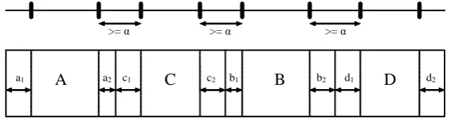
In particular, as a part of the process of folding, the ‡at sheets must be prepared by "scoring" them along the fold lines, which is achieved by knives mounted on a bar. Due to technical lim-itations, the knives cannot be placed at an arbitrary distance to each other, but their distances have to exceed a certain minimum ₂R+ (typically, could be about 70mm in practice). This implies that a given pattern of ‡at boxes as a possible outcome of the …rst stage of the production process is feasible for the second stage only if the boxes can be aligned in a way such that the scores of adjacent boxes are separated by the minimum distance required. The following diagram (Figure 1) illustrates this setting for a possible production pattern that is made up by four (not necessarily di¤erent) boxes A, B, C and D:

A

a2

C

B

D

a1 c1 c2 b1 b2 d1 d2

>=α >=α

[image:10.595.170.492.444.531.2]

>=α

Figure 1: Feasible alignment of boxes I

(11)

[image:11.595.170.492.156.251.2]

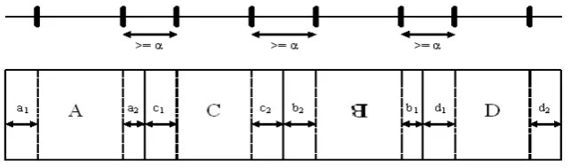
Further combinatorial options arise from the fact that the boxes, when being aligned, can also be rotated by 180o_{, as illustrated in Figure}₂ _{where due to rotating box B, the minimum} score separation constraint is satis…ed ifa2+c1; c2+b2;andb1+d1 :

Figure 2: Feasible alignment of boxes II

Given such a setting, the MSSP consists in determining whether or not a certain set of n boxes can be aligned in an order (possibly also by rotating some of the boxes) such that between each pair of boxes the minimum distance requirement is met. As the number of possible arrangements of the boxes including rotations is O(n₂!2n₎_{- the factor} 1

2 arises due to symmetry - complete enumeration can easily lead to a practically unmanageable combinatorial explosion. (Even in the case of only10boxes, a typical value in practice, this would amount to calculating about1:858 109 _{possible combinations for each candidate production pattern, of} which there can be several thousands in the context of generating columns for solving the cutting stock problem.) Though in practical applications, a pattern that turns out to be infeasible in terms of the MSSP is not entirely useless and can still be employed for manufacturing boxes by running the scoring machine at a slower pace, such a situation would cause considerable costs. Therefore, infeasible patterns must be singled out at an early stage before the cutting stock problem is addressed, and be penalised.

In view of this, it must be considered a practically relevant open combinatorial problem to develop an algorithm that, at least as a heuristic for a large percentage of possible production patterns, can quickly determine if a certain arrangement of boxes is (in)feasible in terms of the MSSP, and explicitly generate such an arrangement if this exists at all.

(12)

(13)

2

Two ways of modelling the MSSP

The aim of this section is to provide a precise de…nition of the Minimum Score Separation Problem by de…ning it in two di¤erent ways: …rst, by describing it as a variant of the so-called "Travelling Politician Problem" as proposed by Goulimis (2004), and second, alternatively, by representing it as a speci…cally constrained Hamiltonian Path Problem on what we will later call a "threshold graph". The di¤erent notions underlying these two de…nitions will be illustrated by giving two di¤erent MIP representations of the problem. As a point of departure, we will start with a de…nition of the Hamiltonian Path Problem on an undirected graph and its general MIP representation as a Travelling Salesman Problem (TSP).

2.1

Starting point: the Hamiltonian Path Problem as a TSP

In the following, letG(N; E)be a (…nite)undirected graph without loops and multi-edges. We will denote its set ofnodes byNG=f1;2; :::; ng N and its set ofedges byEG NG NG. It will be assumed thatEG6=?throughout the text.

De…nition 1 (Hamiltonian Path Problem)

Let G(N; E) be an undirected graph with a node set NG =f1;2; :::; ng N and a set of

edgesEG NG NG. Then the Hamiltonian Path Problem consists in …nding a path

i1 i2 i3 ::: in 1 in

with i1; i2; i3; :::; in 1; in 2 NG and (ik; ik+1) 2 EG for all k = 1;2; :::; n 1, where every

nodeik 2NG occurs in the path once.

By introducing a dummy nodei= 0, a Hamiltonian Path Problem can routinely be modeled as a TSP. The resulting TSP has constant cost coe¢ cients c := (0;0; :::;0) and is de…ned on the extended graphG0₍_{N; E}₎_{, with the new node set being given by}_N_G₀ _:=_N_G_{[ f}₀_g_{and the}

new edge set byEG0 :=E_G[ f0g N_G[N_G f0g.

(14)

minimize0 (1)

subject to X j;j6=i

xij = 1for alli2NG0 (2)

X

i;i6=j

xij = 1for allj2NG0 (3)

yij nxij for allj2NG0; i6=j (4)

X

j>0

y0j =n (5)

X

i;i6=j yij

X

k;k6=j

yjk= 1for allj2NG0 f0g (6)

xij ij for alli; j2NG0; i6=j (7)

xij2 f0; 1g; yij 0for alli; j2NG0; i6=j (8)

In this formulation, constraints (2) and (3) represent the assignment relaxation of the TSP. The "‡ow" yij imposed by constraints (4); (5) and (6) ensures the elimination of subtours. This is achieved by requiring the tour to start at the dummy node with an initial ‡ow of n units on the …rst edge, from which one unit is consecutively "dropped" at each node along the tour until the ‡ow …nally becomes zero. (In the case of several subtours instead of one "full" tour, the subtours without the dummy node would have no initial ‡ow according to(5)so that consecutively dropping a ‡ow at each node along the subtour would lead to a violation of (6)

at the node where the subtour is completed.) Constraints (7) …nally impose the structure of the graph on the model.

2.2

First approach: the MSSP as a Travelling Politician Problem

(15)

[image:15.595.175.488.310.436.2]

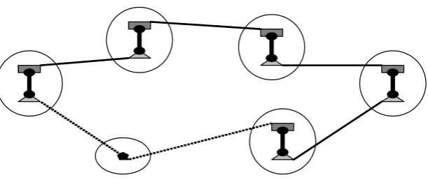
Figure 3 illustrates this problem forn= 5constituencies, with the single node in the ellipse being a dummy node that models the way back to the point of departure. Of course, the general TPP could also be depicted, analogously to the general TSP, without a dummy node, but with a direct way back to the starting point instead. However, as our description here is ultimately intended as a means to represent the MSSP, a dummy node has been included in the diagram. In terms of the MSSP, the di¤erent constituencies representn= 5di¤erent boxes that have to be arranged in a certain order, namely as a path that covers all boxes (all constituencies). The two cities in each constituency denote the two possible ways of including a box ("regular", and after a180o_{rotation) in the alignment. A feasible arrangement of boxes then consists of a} path that passes through all constituencies exactly once. (The dummy node in the ellipse has no representational value in the MSSP as such and just ensures that the path is extended to a tour such that we can illustrate this setting down below by building upon the MIP representation of a TSP.)

Figure 3: The MSSP as a Traveling Politician Problem

Let us now formalise Goulimis’ approach. We can denote the n boxes by two nodes each (for both ways of placing the box into the alignment) such that we obtain a node set NG =

(16)

This yields the following formal de…nition of the MSSP on a directed graph:

De…nition 2 (Minimum Score Separation Problem - Approach 1)

LetG(N; A)be a directed graph with the even node set NG=f1;2; :::;2n 1;2ng, 2R+ a positive number (a "minimal value") and vp:NG!R+ withp2 f1;2g a symmetric pair of "value functions" that assigns two positive numbersv1(i) andv2(i)to every node i2NG such

that the symmetry condition

v1(2k 1) =v2(2k)andv2(2k 1) =v1(2k)for allk= 1;2; :::; n

holds. Moreover, let the edge set of the graph be de…ned by the adjacency condition AG:=f(i; j)with v2(i) +v1(j) j

i= 2k_^j₆= 2k 1 ori= 2k 1_^j₆= 2kfor somek= 1;2; :::; n_g:

Then the MSSP consists in deciding whether there exists onGa subpath that contains exactly

one node out of each of the node subsets_f2k 1; k_g for allk= 1;2; :::; n.

To state this de…nition di¤erently: The perspective involved in this approach implies (due to the symmetry between the odd and the even nodes) that the MSSP is feasible if the graph just de…ned can be partitioned into two subsetsSand

_

S of nodes of equal cardinality such that (a) for each k= 1;2; :::; neither (2k 1)₂S and (2k)₂S or (2k)₂S and(2k 1)₂S and that (b) there exists a Hamiltonian path in one subset (and, due to symmetry, consequently also in the other subset). Conversely, if such a partition does not exist, the MSSP is infeasible. In the diagram above, when leaving aside the dummy node and the dotted edges, this partition is represented by the set of the connected nodes on one side and the set of the unconnected nodes on the other side. Because of the symmetry between "regular" boxes and their rotated counterparts, the path drawn in the diagram ensures that there exists also a path covering the unconnected nodes, and this in the same order of constituencies.

We can illustrate this de…nition of the MSSP by a MIP formulation gained from the TSP representation based on the Hamiltonian path property of the subsets. This means the following TSP is feasible if and only if there exists a subtour in the graph that covers all and only all of the nodes of a subset S of which for each k = 1;2; :::; n either the node (2k) or the node

(2k 1)is an element. Again, corresponding to the general TSP model for Hamiltonian paths above, we have to introduce a dummy node0(the one already depicted in …gure2above) and de…ne the extended graphG0₍_{N; A}₎_{, with the new node set given by}_N

(17)

minimize0 (1)

subject to X j;j6=2i 1;j6=2i

(x2i 1;j+x2i;j) = 1for alli2NG0 f0g (2a’)

X

j>0

xj0= 1 (2b’)

X

i;i6=2j 1;i6=2j

(xi;2j 1+xi;2j) = 1for allj2NG0 f0g (3a’)

X

j>0

x0j= 1 (3b’)

X

j;j6=i xij

X

j;j6=i

xji= 0for alli2NG0 f0g (9)

yij nxij for alli; j2NG0; i6=j (4’)

X

j>0

y0j =n (5’)

X

i;i6=j yij

X

k;k6=j yjk=

X

i;i6=j

xij for allj 2NG0 f0g (6’)

In this formulation, constraints(2a0);(2b0);(3a0)and(3b0)are the equivalents of the assignment relaxation constraints of the TSP above. Constraints(2a0₎_and ₍₃_a0₎_{refer to all nodes}

repre-senting a box. Corresponding to the set S NG0 that, for eachk= 1;2; :::; n, contains either the node(2k)or the node(2k 1)as an element, only half of the nodes (namely one for each box) must be assigned to one successor and one predecessor. Constraints(2b0₎_and₍₃_b0₎_make

sure that the dummy node de…nitely is included in the tour with one successor and one prede-cessor. However, in contrast to the general MIP formulation of the Hamiltonian Path Problem, these assignment relaxation constraints must be complemented by constraints (9). Without

(9), constraints(2a0₎_and₍₃_a0₎_{would allow some nodes to have either only predecessors or only}

successors. This is avoided by forcing both sums in (9) to either the value 1 or the value 0

for alli₂NG0 f0g. Doing so ensures that all nodes representing boxes have either (a) both a predecessor and a successor, or (b) neither a predecessor nor a successor, i.e. the nodes are either fully included in or entirely excluded from the tour.

The ‡ow constraints for the elimination of inappropriate subtours (40₎_; ₍₅0₎ _and ₍₆0₎_have

been only slightly modi…ed compared to the TSP above. Note however that, despite_jNG0j=

2n+ 1here, constraints(40₎_and₍₅0₎_{still have the constant}_n_{on their right-hand sides because}

(18)

regarding the constraints (60₎ _{takes into account that a node may be used for the subtour or}

not at all. If and only if a node is part of the tour to be found, the right-hand side of(60₎_equals

1and a unit of the ‡ow is "dropped" at the node. Otherwise, the right hand side equals0 and the corresponding node j is neutral with respect to the ‡ow that enforces the elimination of subtours. Finally, constraints(7)again impose the structure of the graph on the model.

2.3

Second approach: the MSSP as a Twin-Constrained Hamiltonian

Path Problem

We will now introduce an alternative approach to the MSSP, which is more intuitive in so far that (as the reader will also observe in terms of notational e¤ort) it goes down more "naturally" on the basis of the concept of Hamiltonian Paths. Still, we model each box by two nodes and look for a certain path connecting the nodes. However, while in the …rst approach the two nodes for each box represent the two possible positions of a box in the alignment ("regular", or rotated), here the two nodes correspond to the left and the right sides of the boxes. This means that if a "regular" box is described by a pair(i; j)₂NG NG, its rotated counterpart is denoted as(j; i). We will call the two nodes that make up a box "twin nodes" in the following. Analogously to the preceding subsection, we could imagine the left hand sides of the boxes being represented by the odd node numbers in the node set, and the right hand sides by the even numbers, but we will not require this in the following because the algorithm for the MSSP to be developed later will permute the order of nodes anyway. This is why we will remain more ‡exible and introduce a "twin node function" as a bijective function b : NG ! NG from the set of nodesNG onto itself that associates each nodei2NGwith its twin node t:=b(i)2NG (consequently we have b(b(i)) = b(t) = i). Then, if a node i represents one side of a certain box, the nodeb(i)represents the other side of this box, and it does not matter, ifiis the right or the left side of the box, or if the box is included in the alignment in a "regular" or a rotated fashion. Note that the notion of "twin nodes" here does not imply that two twin nodes are adjacent to the same set of other nodes because the two sides of a box could di¤er with respect to the other boxes they can be placed next to. In this model, "twins" are closely attached to each other, but not perceived to be necessarily identical, so to speak.

Similarly to the previous subsection, we will denote the minimum knife distance by a certain positive ₂_R₊ and introduce a "value function" v to model the widths of the left and right sides of the boxes. However, since we model each side of a box separately from the other side in this alternative approach, one value functionv:NG!R+su¢ ces here, and we can do without a "symmetry condition" of the kind imposed on the pair of value functions in the previous subsection. On this simpler basis, two nodes i; j ₂ NG ful…l the minimum score separation constraint, i.e. are adjacent in the graphG, if and only ifv(i) +v(j) provided that they do not belong to the same box, i.e. j₆=b(i).

(19)

boxes into halves), both nodes modeling a box must …nally be part of the path that represents the alignment of boxes. In other words: this way of describing the MSSP, in contrast to Goulimis’ approach, does not require a certain subpath in a partition of nodes for a feasible solution, but instead a (complete) Hamiltonian Path, which (by de…nition) covers all nodes of the graph. In this perspective, the MSSP …nally turns out to be a "normal" Hamiltonian Path Problem on a graph given by the speci…c adjacency condition v(i) +v(j) for all nodes j₆=b(i), with the only additional requirement being that each node has its twin node either as its successor or its predecessor ("twin node condition").

This gives rise to the following de…nition.

De…nition 3 (Twin-Constrained Hamiltonian Path Problem)

Let G(N; E) be an undirected graph with node set NG = f1;2; :::; ng N , a set of edges

EG NG NG, andb:NG!NG a bijective function that associates every nodei2NG with

a "twin node" t:=b(i)₂NG,t6=i. Moreover, let G0 be a graph derived from Gby NG0 :=N_G andE_G0 :=E_G[ f(i; j) :i=b(j)g.

Then the Twin-Constrained Hamiltonian Path Problem on G with respect to b consists in

deciding whether there exists onG0 a Hamiltonian path of the form

i1 b(i1) i2 b(i2) ::: in b(in),

i.e. a Hamiltonian path in which every node is either predecessor or successor of its twin node ("twin node condition"). Gis called the underlying graph and bthe twin-node function of the Twin-Constrained Hamiltonian Path Problem.

Note that, due to the bijectivity of the twin function b, the twin node condition actually describesall possible types of paths in which every node is either predecessor or successor of its twin node. Obviously, equivalent formulations of this condition would be, for example, also

b(i1) i1 b(i2) i2 ::: b(in) in, and i1 b(i1) b(i2) i2 i3 b(i3) ::: b(in) in.

The setting of a twin-constrained Hamiltonian path is illustrated for an MSSP withn= 5

boxes in Figure4, in which the two nodes that share a circle (the triangle and the rectangle) correspond to the same box (imagine the rectangles as their right sides and the triangles as their left ones, "normal" position given). The inseparability of the twin nodes in the model is re‡ected by the bold lines (edges) connecting triangles and rectangles such that any Hamiltonian Path must either enter a circle at the side of the triangle and proceed to the rectangle, or vice versa. Again, the ellipse represents a dummy node to turn the Hamiltonian Path Problem into a TSP.

(20)

[image:20.595.179.485.102.231.2]

Figure 4: The MSSP as a twin-constrained Hamiltonian path problem

entities for representing rotated boxes. Despite this e¤ort of doubling the mathematical struc-ture, any solution to the MSSP (if there exists one at all for a certain instance) will use only half of the nodes in the model. Such a structural redundancy is theoretically unsatisfying and suggests looking for a more straight forward approach (also in view of the classical method-ological principle of "Occam’s razor"). This is why our alternative approach models each side of a box separately from the corresponding other side and additionally imposes the "twin node condition". In proceeding in this way, we can describe every solution to the MSSP readily as a Hamiltonian Path in terms of all boxes. Moreover, apart from a certain elegance involved in this description, this perspective of looking at the MSSP opens up a ‡exible way to exploit the adjacency conditions of the graph for each node separately because we do not have to care about both sides of a box at the same time - at least not in the …rst instance. In particular, modeling the sides of the boxes separately leads to a "threshold graph", the properties of which can fruitfully be exploited for …nding a solution to the MSSP. Finally, the algorithm gained in this way shows a surprisingly e¤ective behaviour, which ultimately justi…es this perspective on the MSSP.

Having presented the ideas underlying our alternative approach, we summarize the second model of the MSSP in the following formal de…nition:

De…nition 4 (Minimum Score Separation Problem - Approach 2)

LetG(N; E)be an undirected graph with an even set of nodes NG=f1;2; :::;2n 1;2ng

N , and b : NG ! NG a twin node function. Moreover, let 2 R+ a positive constant (a

"minimal value") and v : NG ! R+ be a "value function" that assigns a positive number to

each node. The edge set of the graph EG NG NG.be de…ned by the adjacency condition

(i; j)₂EG:,v(i) +v(j) for all i; j2NG; j6=i.

Then the Minimum Score Separation Problem (MSSP) consists in deciding if there exists a

(21)

Finally, we will illustrate also this de…nition of the MSSP by a MIP formulation gained from the TSP presentation of the Hamiltonian Path property of a feasible solution to the MSSP. The reader will observe that this approach comes much closer to modeling the general Hamiltonian Path Problem than Goulimis’approach does. Again, corresponding to the general TSP model for Hamiltonian Paths above, we have to introduce a dummy node 0 (the one already depicted in …gure3), and de…ne the extended graphG0(N; E), with the new node set given by NG0 :=N_G[ f0g and the new edge set byE_G0 :=E_G[ f0g N_G[N_G f0g. Also analogously, introducing for all nodesi; j₂NG0; i6=j;the binary variablesx_ij, the continuous ‡ow variables yij, and the binary constants ij = 1 :, (i; j) 2EG0 yields the following MIP approach to the MSSP.

minimize0 (1)

subject to X j;j6=i

xij = 1for alli2NG0 (2)

X

i;i6=j

xij = 1for allj2NG0 (3)

xi;b(i)+xb(i);i= 1 for alli2NG0 f0g (10)

yij 2nxij for alli; j2NG0; i6=j (4”)

X

j>0

y0j= 2n (5”)

X

i;i6=j yij

X

k;j6=k

yjk= 1for allj2NG0 f0g (6)

In contrast to the …rst approach formalised above on the basis of Goulimis’ suggestions, our formulation requires only minor changes of the original MIP for the Hamiltonian Path Problem. The assignment relaxation constraints(2),(3)and the subtour elimination constraint(6)remain the same as in the original problem. The only signi…cant di¤erence here is the introduction of the additional "twin node constraints"(10):Complementing the assignment relaxation constraints, they ensure that each node has its twin node either as its predecessor or its successor. The subtour elimination constraints (400₎ _and ₍₅00₎ _{can be kept almost unchanged, with the only}

(22)

3

The MSSP, Hamiltonian paths, variants of the TSP and

complexity theory

We have seen in the previous chapter that our approach of modelling the Minimum Score Sep-aration Problem leads to a speci…c type of Hamiltonian path problem and a speci…c variant of the Travelling Salesman Problem. This chapter explores in more detail of how the Mininum Score Separation Problem is related to existing research about these problems, namely to re-search about the Hamiltonian Path Problem, the Travelling Salesman Problem, the Clustered Travelling Salesman Problem, and the Generalised Travelling Salesman Problem. Moreover, it addresses the question of the complexity of the MSSP. In doing so, we will proceed from the most speci…c case, which is the Hamiltonian path problem, to the most general case, namely the Generalised Travelling Salesman Problem. We begin with some preliminary remarks on the notation used in this thesis.

3.1

Notation

In the remainder of this paper, we will mostly follow Schrijver’s notation (Schrijver 2003). Whenever speci…c aspects of threshold graphs are concerned, we apply Mahadev’s and Peled’s notation, who have written the major source on this topic (Mahadev and Peled 1995).

LetG(N; E)be a (…nite and simple)undirected graphwithnode set NG=f1;2; :::; ng N

and edge set EG NG NG It will be assumed thatEG 6=? throughout the text. As, in

most cases, we prefer to denote edges by pairs of nodes (instead of using the set notation_fi; j_g, which can often be found in the case of undirected graphs), we will always take for granted that

(i; j)₂EG ,(j; i)2EG when using this notation. A graphG(N; E)is calledcomplete i¤ we have EG=NG NG. Given two graphsG(N; E)andG0(N; E)with

NG0 N_G andE_G0 E_G,

the graphG0 _{is called a}_{subgraph of} _G_and_G_{is said to} _contain_G0_{. For}

NG0 :=P $N_G andE_G0 :=E_G\P P, the graphG0(P; E)is called thesubgraph of Ginduced by P.

Apath in an undirected graphG(N; E)is a sequence

(i0; e1; i1; :::; en; in)

wherei0; i1; :::; in 2NG are distinct nodes ande1; e2; :::; en 2EG edges such thatek is an edge that connects the nodesik 1 andik. We will calli0andin theend nodes of the path and say that the path connects the nodesi0; i1; :::; in 2NG. A sequence

(i0; e1; i1; :::en 1; in 1; en; in)

(23)

fe1; e2; :::; eng E or the corresponding order of nodes

i0 i1 ::: in 1 in.

A graphG is said to beconnected if for any two of nodes i0; in 2NG there exists a path the end nodes of which are i0 andin, and it is calledHamiltonian if there exists a cycle that connects all nodes in NG. Such a cycle is called aHamiltonian cycle. By removing one edge from a Hamiltonian cycle, we obtain aHamiltonian path.

For any nodei₂NG, the subset of nodesN(v) NGis called aneighbourhood of the node iifN(i)contains all nodes that are adjacent toi, i.e.

N(i) :=_fj₂NG : (i; j)2EGg:

Theclosed neighbourhood N[i] NGof a node i2NG is the union ofiand the

neighbour-hood ofi, i. e.

N[i] :=N(i)_{[ f}i_g.

A node is calledisolated if its neighbourhood is empty, anddominating if its closed neigh-bourhood is the entire set of nodes.

A subset of nodesS NG is astable set wheni =2N(j)for all nodesi; j2S, and a subset K NG is called aclique wheni2N(j)for all nodesi; j2K.

Apreorder is the pair(P;%)of a setP and a binary relation%onP when the two following

properties hold:

(i)p%pfor allp₂P , (re‡exivity)

(ii) (p1%p2)^(p2%p3))(p1%p3)

for allp1; p2; p32P . (transitivity)

We will say the preorder istotal i¤ all nodes can be compared with respect to the preorder, i. e.

p1%p2or p2%p1 for allp1; p22P. De…ning a binary relation%on the set of nodesNG by

i%j:_,N[i] N(j)for alli; j₂NG,

clearly yields a preorder, which will be called thevicinal preorder of G(and is not total in the general case). If i%j, we will call the nodei greater thanj, and j smaller thani. (Note that it is possible to have bothi%j andj%i, which is equivalent toN(i)_nfj_g=N(j)_nfi_g.)

The cardinality of the neighbourhood of a nodei is called itsdegree, denoted by dg(i) :=_jN(i)_j.

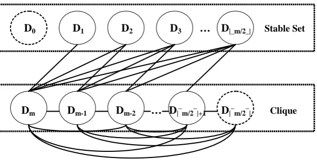
Given the family 1< 2< ::: < m 1< m of distinct positive degrees of a graphG, and

0:= 0 (even if there are no isolated nodes in the graph), we de…ne the family of sets Dk:=fi2NG:dg(i) = kgfor allk= 0;1; :::; m

and call

(24)

thedegree partition of G.

For a graphG(N; E)the relationM EG NG NGis called amatching i¤ the relation is (i)symmetric, i.e. (i; j)₂M implies(j; i)₂M for alli; j₂NG, (ii)functional, i.e. (i; j)2M implies(i; k)₂= M for all i; j; k ₂NG, k =6 j, and (iii)(i; i)2= M for all i2 NG. A matching M is said to be amaximum cardinality matching if_jM_j _jM _jfor all matchingsM E. If a matching is aleft-total relation, i.e. for alli₂NG there exists a j2NG such that(i; j)2M, the matching is calledperfect.

3.2

Hamiltonian paths and alternating Hamiltonian paths

In this section we will address the relationship of the MSSP to research on the Hamiltonian Path Problem and some of its generalisations. As mentioned in the …rst chapter, for a given undirected graphG(N; E)a Hamiltonian path is a path

i1 i2 i3 ::: in 1 in withi1; i2; i3; :::; in 1; in 2NG and

(ik; ik+1)2EG for allk= 1;2; :::; n 1,

such that every nodeik 2NG occurs in the path exactly once.

We will speak of aHamiltonian cycle i¤ the …rst and the last node of the path are identical, and a graph with at least one Hamiltonian cycle is said to beHamiltonian.

The problem of …nding a Hamiltonian path or cycle, while being named after Hamilton (1858), was already described in an earlier paper by Kirkman (1856), who discussed a planar graph that is not Hamiltonian (see Biggs, Lloyd and Wilson (1976) for details on the history of this problem). Since these early publications, more than one thousand papers have been published, providing theoretical insights, algorithms or applications of the problem. Among the theoretical insights there are criteria for Hamiltonicity and non-Hamiltonicity based on certain characteristics of a graph (such as connectedness, toughness or the number of edges), for example, stochastic analyses on the frequency of Hamiltonian graphs, theorems on the Hamiltonicity of graphs that do not contain speci…c subgraphs, and results on the number of di¤erent Hamiltonian cycles that might exists for a particular graph. An overview of the vast amount of literature on these and related topics can be found in Bermond (1978), Gould (1991) and Gould (2003).

(25)

Bruckstein (1999), for example), while others are exact algorithms that give a de…nite answer to the question of whether a given graph is Hamiltonian (such as Shufelt and Berliner (1994), for example). While the latter come with the disadvantage of a long computational time in the worst case, the former might not …nd a de…nite answer on the Hamiltonicity of an input instance (cf. Shields, 2004, for more details on some of the algorithms).

Additionally, research has led to algorithms for speci…c classes of graphs that can decide on the Hamiltonicity of a graph in a comparably short amount of computational time ("polynomial time", to be precise, see section 4 of this chapter). Among the speci…c classes of graphs for which such an e¢ cient algorithm exists there are, for example, proper interval graphs (Bertossi, 1983), interval graphs (Keil, 1985), circular-arc graphs (Shih, Chern and Hsu, 1992), threshold graphs (Mahadev and Peled, 1994, see also chapters 4 and 5 of this thesis for more details), graphs without "claws" and "nets" as subgraph (Brandstaedt, Dragan and Koehler, 2000), distance-hereditary graphs (Hung and Chang, 2005), strongly chordal graphs that do not contain the subgraphs

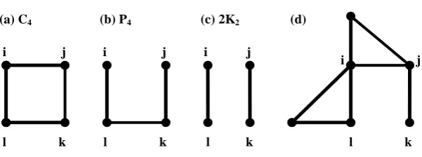
G1(N; E1)andG2(N; E2)

with the (common) node setN :=_fa; b; c; d; e_g and the edge sets E1:=f(a; b);(a; c);(b; c);(c; d);(c; e)g,E2:=E1+f(d; e)g

and have an order of at least 5 (Abueida and Sritharan, 2006), and quasi-adjoint graphs (Blazewicz, Kasprzaka, Leroy-Beaulieuc and de Werra, 2008). Note that the references given for e¢ cient algorithms here, refer to the …rst published paper to tackle algorithmically the question of the Hamiltonicity of a particular class of graphs. For many of these graph classes, later research led to the development of improved algorithms that solve the Hamiltonian cycle (or path) problem with less computational e¤ort.

Apart from the result on recognizing Hamiltonian threshold graphs, to which we will come back in chapter 5 of this thesis, going more into the details of these streams of research on the Hamiltonicity of graphs is not necessary for discussing our problem, the MSSP. As mentioned in the previous chapter, the MSSP is a Hamiltonian path problem with one additional type of constraint, namely the constraints that each node must have its twin-node as a successor (or predecessor) in the Hamiltonian path. If we would like to arrive at an algorithm that exploits the speci…c structure of the MSSP, we can not expect the results of the research on the (ordinary) Hamiltonian path or cycle problem to be particularly helpful for us. For this reason, let us turn to a variant of the problem of recognizing Hamiltonian graphs that has a more speci…c structure: the problem of …ndingalternating (Hamiltonian) paths and cycles.

De…nition 5 (Alternating Hamiltonian cycles and paths on 2-edge-coloured graphs)

For a given graphG(N; E), we colour some edges "red" and some edges "blue". The graph

G is said to have an alternating Hamiltonian cycle (path) if there exists a Hamiltonian cycle

(path) onGsuch that successive edges di¤ er in colour. Gis said to be alternating Hamiltonian

(26)

Remark 6 We note that the twin-constrained Hamiltonian path problem, and hence the MSSP, is obviously a special case of the problem of …nding an alternating Hamiltonian path, as we can imagine the edges of our underlying graphGas "blue" edges and the edges(i; b(i))that connect a pair of twin nodes as "red" edges.

The following proposition attributed to Häggkvist (1979) states that, in a certain sense, the problem of …nding an alternating Hamiltonian cycle (path) on a 2-edge-coloured graph generalizes the problem of …nding an ordinary Hamiltonian cycle (path).

Proposition 7 (Reducibility of Hamiltonicity to alternating Hamiltonicity)

An algorithm that can decide on the alternating Hamiltonicity of graphs is able to decide on the Hamiltonicity of graphs.

Proof. For a given (uncoloured) graph G(N; E)we de…ne a new graph G0 _{by (i) introducing}

for each edge (i; j) ₂ E two new nodes k and l, (ii) replacing (i; j) by the four edges (i; k),

(k; j), (i; l) and (l; j), and (iii) colouring the edges (i; k) and(l; j)"red", while colouring the edges(k:j)and(i; l)"blue". If we can …nd an alternating Hamiltonian path (cycle) onG0_{, we}

just have to replace the four edges (i; k), (k; j), (i; l) and(l; j)by the original edge(i; j) and remove the nodesk andl in order to construct a Hamiltonian path (cycle) onG. Conversely, any Hamiltonian path (cycle) onGobviously corresponds to an alternating Hamiltonian path (cycle) onG0_.

The concept of alternating paths goes back, as do an astonishing number of graph theoretical problems, to Petersen (1891). (See also Mulder (1992) for a discussion of Petersen’s results in the light of contemporary graph theory.) The problem of alternating Hamiltonicity is likely to have …rst been introduced by Bankfalvi and Bankfalvi (1968), going back to a problem stated by Erdös (cf. Bang-Jensen and Gutin, 1997). In their paper, Bankfalvi and Bankfalvi gave a criterion according to which the Hamiltonicity of a2-edge coloured complete(!) graph with an even node set depends on the sum of the degrees of the nodes in certain pairs of disjunct subsets of the node set. Apart from this theorem, three other early results on alternating cycles (paths) were presented in Daykin (1976), Bollobás and Erdös (1976) and Chen and Daykin (1976), who gave criteria for the existence of alternating cycles of certain lengths for a complete graph no node of which is incident to more than kedges of the same colour, provided that the number of nodes exceeds a certain threshold depending onk.

(27)

coloured graph, subgraphs other than paths and cycles (such as trees, or node partitions with speci…c properties) such that all edges have the same colour or di¤er in colour (see Kano and Li, 2008, for a survey).

The majority of this stream of research on alternating subgraphs focusses almost exclusively on graphs that are complete and/or bipartite, in particular those papers that deal with Hamil-tonian paths (cycles). As will become clearer in section 4 of this chapter and in section 3 of chapter 5, we are well advised to exploit the speci…c structure of the graph Gunderlying our MSSP according to De…nition 3. Therefore we cannot expect to bene…t from more details of the literature on alternating paths (cycles) and we will stop our survey on this body of research here.

3.3

The Travelling Salesman Problem and generalisations

The Hamiltonian path problem of the previous chapter can be generalized to the Travelling Salesman Problem (TSP).

De…nition 8 (Travelling Salesman Problem - TSP)

For an undirected graphG(N; E)and a ("cost") functionc:E_!Rthe Travelling Salesman Problem consists in …nding a Hamiltonian cycle

i1 i2 i3 ::: ijNGj i1, with ik 2NG for1 k jNGj

onGsuch that

P

1 k jNGj

c[(ik 1; ik)] +c[(i_jNGj; i1)]

is minimal.

Remark 9 (1) In the literature the TSP is often de…ned only for complete graphs. This is

not a restriction as we can transform a TSP on an arbitrary graph G(N; E) into a TSP on a

complete graph by de…ning c(f) := P

e2E

c(e) + 1for allf ₂(NG NG) E.

Then the TSP on the graphGhas a solution if and only if we have

P

1 k jNGj

c[(ik 1; ik)] +c[(ijNGj; i1)]

P

e2E c(e)

for an optimal solution of the TSP on the complete graph.

(28)

The TSP was probably …rst stated in a German handbook for traveling salesmen (Voigt, 1831; cf. Müller-Merbach 1983) and found its way into the mathematical literature in the 1930s (see Ho¤man and Wolfe (1985) and Schrijver (2003) for more details on the history of the problem). Since then, it has become one of the most thoroughly investigated combinatorial problems. Detailed surveys on the development of research on the topic, with respect to the mathematical structure of the TSP, its applications as well as algorithms for solving it, can be found in Bellmore and Nemhauser (1968), Lawler, Lenstra, Rinnooy Kan and Shmoys (1985), Jünger, Reinelt and Rinaldi (1995), Burkhard, Deineko, van Dal, van der Veen and Woeginger (1998), and Gutin and Punnen (2002). Additionally, Gutin (2009) provides an excellent intro-ductory overview, and Orman and Williams (2004) compare various di¤erent ways of modelling the TSP as an Integer Programming problem.

Obviously, our MSSP is not immediately a TSP because the MSSP requires us to …nd a Hamiltonian path that satis…es the additional constraint that the successor (or predecessor) of each node is its twin-node. There are several generalisations of the TSP in the literature that originate from adding a speci…c type of constraint to the TSP. Among these there are the TSP with time-windows, in which some nodes have to be visited during a certain period of time (see Dumas, Desrosier, Gelinas and Solomon (1995), for example), the TSP with precedence constraints, in which certain nodes can only be visited after certain other nodes have been visited (see Balas, Fischetti and Pulleyblank (1995), for example), and the TSP with pickup and delivery, in which each node is associated with a "pickup quantity" and a "delivery quantity" and a feasible Hamiltonian cycle satis…es the additional condition that the quantity transported along the cycle does not exceed a certain capacity (see Gendreau, Laporte, Vigo (1999), for example). A large variety of further generalisations can be found in the book chapters by Balas (2002), Barvinok, Gimadi and Serdyukov (2002), Fischetti, Salazar-Gonzáles and Toth (2002), and Kabadi and Punnen (2002).

A particular one among these generalisations of the TSP is of interest for us as the MSSP can be considered a direct subcase of it: the Clustered Traveling Salesman Problem (CTSP). The CTSP was introduced into the literature by Chisman (1975). A short overview of the literature and of several applications can be found in Laporte and Palekar (2002).

De…nition 10 (Clustered Traveling Salesman Problem - CTSP)

For an undirected graphG, a partition of the node set into sets ("clusters")Ni,1 i n,

with N1+N2+:::+Nn = NG and a function c : NG NG ! R, the Clustered Traveling

Salesman Problem consists in …nding an optimal solution of the TSP onGunder the additional

(29)

Remark 11 (1) Also the CTSP is typically de…ned on a complete graph in the literature.

Remark9(1)applies analogously.

(2) The twin-constrained Hamiltonian path problem on a graph G with respect to the twin

node function b (and hence the MSSP) can directly be stated as an CTSP on a graph G0 that

results from adding to the underlying graphGa twin-node pair of dominating nodes and

parti-tioning the node set of G0 into clusters of cardinality2 such that each cluster contains one of

the nodesi₂NG0 of the graph and its twin-node b(i). Then the twin-constrained Hamiltonian

path problem on G with respect to b is feasible if and only if the CTSP on G0 _{has a feasible}

solution.

Despite its speci…c structure of the node set and the additional constraint that all nodes within a cluster must be visited consecutively, the CTSP is eventually equivalent to the TSP in the sense that any instance of a TSP can be transformed into an instance of the CTSP, and vice versa.

Proposition 12 (Reducibility of CTSP to TSP and vice versa)

LetG(N; E)be an undirected graph, a cost function c:E_!R, and a partition N1+N2+

:::+Nn =NG for the CTSP. An algorithm that is able to solve the TSP to optimality is also

able to solve the CTSP to optimality, and vice versa.

Proof. An instance of the TSP can trivially be transformed into an instance of the CTSP by partitioning the node set into clusters Ni with jNij= 1 for1 i jNGj. Conversely, an instance of the CTSP can be transformed into an instance of the TSP in the following way. We add to the cost of all edges between clusters the constant

M := P

e2E

c(e) + 1.

As the CTSP hasnclusters, a feasible solution of the CTSP must contain n inter-cluster edges. Therefore, if and only if the TSP on Gwith the rede…ned cost function has a solution with

P

1 k jNGj

c[(ik 1; ik)] +c[(i_jNGj; i1)] (n+ 1)M 1,

the CTSP with the original cost function has a feasible solution and the Hamiltonian cycle found by the TSP algorithm is also the optimal solution of the CTSP.

Remark 13 Note that a case parallel to the preceding proposition would be a transformation of the alternating Hamiltonian path problem into a Hamiltonian path problem. However, such a transformation is not possible because we were able to transform the CTSP into the TSP only by virtue of a rede…ned cost function.

(30)

as doing so would (at least partly) disregard the particular cluster structure of the CTSP. Therefore speci…c algorithms and heuristics for tackling the CTSP have been developed, which can be found in Jongens and Volgenant (1985), Arkin, Hassin and Klein (1994), Laporte, Potvin and Quilleret (1997), Renaud and Boctor (1998), Anily, Bramel, and Hertz (1999), Guttmann-Beck, Hassin, Khuller and Raghavachari (2000), and Dinga, Cheng and He (2007). We will not go further into the details of these algorithms here as we have reasons (see the following section) to focus on exploiting both the speci…c structure of the graph underlying the MSSP and the speci…c structure given by the twin-node function two aspects that, to the best of our knowledge, have not been addressed in the literature.

Another variant of the TSP is worth being addressed here due to its close relation with our MSSP: the Generalized Traveling Salesman Problem (GTSP). More details on this problem can be found in Laporte, Asef-Vaziri and Sriskandarajah (1996).

De…nition 14 (Generalized Traveling Salesman Problem GTSP)

For an undirected graphG, a partition of the node set into sets ("clusters")Ni,1 i n,

with N1+N2+:::+Nn = NG and a function c : NG NG ! R, the Generalized Traveling

Salesman Problem consists in …nding a minimum cost cycle on G that passes through each

clusterNi,1 i n, exactly once.

Remark 15 (1)In a di¤ erent version of the GTSP, the minimum cost cycle must pass through each cluster at least once (see Laporte, Asef-Vaziri and Sriskandarajah ,1996).

(2) The GTSP can be reduced to a CTSP by doubling all nodes and rede…ning the cost

functioncin an appropriate manner (see Laporte and Semet (1999) for details). Consequently,

the GTSP can also be reduced into a TSP. Conversely, each TSP can trivially be transformed

into a GTSP by partitioning the node set into clustersNi withjNij= 1for1 i jNGj.

(3)The original model for the MSSP by Goulimis (see chapter2:2) can be seen as a GTSP

with clusters of cardinality2.

(4)More generally, any alternating Hamiltonian cycle problem can be reduced to a GTSP.

For doing so, we replace each node of the alternating Hamiltonian cycle problem by a cluster of nodes. Each node in such a cluster represents a way of visiting the original node such that we arrive at that node via taking a blue edge and depart from that node via a red edge (or vice versa).

(31)

one node, depending on the variant of the problem) from each cluster of the node set partition. Clearly, Network Design Problems are a relaxation of the TSP, while Generalized Network Design Problems are a relaxation of the GTSP. The theoretical relevance of the concepts of the Network Design Problem and the Generalized Network Design Problem lies in the fact that theoretical results (such as polyhedral, algorithmic, and complexity-related results) about these problems can be applied to a variety of subgraph problems, such as the (Generalized) Minimum Spanning Tree Problem (Feremans, C., M. Labbé and G. Laporte, 2002), of which the Network Design Problem and the Generalized Network Design Problem are relaxations.

3.4

Relevant results of complexity theory

In this section we …rst review some de…nitions and results from complexity theory and, in a second step, apply these results to the problems presented in the preceding two sections. Doing so will give us an insight into the computational "di¢ culty" of the twin-constrained Hamiltonian path problem. Our review of de…nitions and results from complexity theory mainly follows the presentation in Johnson and Papdimitrou (1985, pp. 42-58) - albeit not always in the order of their presentation and apart from some references to other sources when we go slightly more into detail. A rigorous formal treatment based on the concept of the Turing machine can be found in Jongen, Meer and Triesch (2004, chapters 18-22), for example.

We begin by distinguishing between two types of problems in the computational complexity of which we are interested.

De…nition 16 (Decision and optimization problems)

(1)A problem that can be solved by an algorithm that produces only a "yes" or "no" answer is called a decision problem.

(2)A problem is referred to as an optimization problem if solving it means …nding an optimal

feasible solution to the problem with respect to some objective function. For a given optimization

problem that is a minimization problem and a given number b, we call the decision problem of

whether there exists a feasible solution to the optimization problem with an objective function

value less than or equal to b the decision problem version of the optimization problem.

(32)

De…nition 17 (O(f(n)-notation and the class of polynomial-time decision problems P)

(1)For a function f :N!R, we say that the running time of an algorithm isO(f(n))i¤

there exists a constantc >0 such that the number of steps that an algorithm needs to solve a

problem for all instances of sizen has an upper bound ofcf(n)ifn is su¢ ciently large.

(2)An algorithm for which such a polynomial function f exists is said to be e¢ cient or a

time algorithm. The class of all decision problems that can be solved by

polynomial-time algorithms is denoted byP.

Remark 18 In this and all following chapters we will equate the input size nwith the cardi-nality of the node set of the graph that our problem is based on, and we will count as one, single (unit time) step all summations, multiplications, and all operations that compare the size of two given numbers (such operations are called elementary arithmetic operations). This simpli-…cation is justi…ed because the number of steps needed for multiplications and comparisons is polynomially bounded by the number of steps needed for summations and we are only concerned with the question of whether there exists, or is likely to exist, an e¢ cient, i.e. polynomial time algorithm for a problem. This simpli…cation also implies that we will disregard the details of how the actual number of steps needed for an elementary arithmetic operation depends on the numerical size of the input data. In line with most of the literature on combinatorial optimiza-tion (cf. Papadimitrou and Steiglitz,1998, chapter 8), it su¢ ces for us to know that this actual number of steps, and the memory space needed for carrying them out, are bounded by a polyno-mial in the numerical size of the input data. More precisely speaking, an algorithm that requires only polynomial time with respect to elementary arithmetic operations and in which the space needed for carrying out each of these operations is bounded by a polynomial in the numerical size of the input data is called strongly polynomial (cf. Schrijver, 2003).

The subsequent de…nition presents two concepts that are important tools for comparing the complexity of two algorithms.

De…nition 19 (Polynomial-time reducibility and polynomial-time transformability)

(1) A problem A is called polynomial-time reducible to a problem B if there exists an

al-gorithm for A that uses an algorithm for B as a subroutine and the algorithm for A runs in

polynomial time if we count each call of the subroutine as a unit time step.

(2) A decision problem A is called polynomial-time transformable to a problem B if A is

polynomial-time reducible toBand the algorithm forAcalls only once the subroutine that solves

(33)

Remark 20 (1) It immediately follows from the de…nition that, if there exists a

polynomial-time algorithm for problemB and problemA is polynomial-time reducible to problem B, there

exists a polynomial-time algorithm for problemA.

(2)It follows also by means of the concept of polynomial-time reducibility that if the value of

the objective function of the optimization problem can be calculated in polynomial time and the numerical size of the optimal solution is bounded by a polynomial in the numerical size of the input data, the decision problem version of an optimization problem can be solved in polynomial time if and only if the optimization problem can be solved in polynomial time.

(3)We note that the property of polynomial-time transformability is transitive.

We now introduce two more classes of problems. The …rst class of problems was introduced by Cook (1971) and Karp (1972), while the second class was …rst described by Edmonds (1965b) who referred to problems in this class as problems with "good characterisations".

De…nition 21 (Polynomial-time nondeterministic decision problems NP) An algorithm that is able to carry out an instruction of the type

goto both label 1, label 2,

i.e. that can carry out arithmetic operations in an exponential number of branches of a search tree in parallel at the same time, is called a nondeterministic algorithm. A nondeterministic

algorithm is said to solve a decision problem with input sizenin polynomial time i¤ there exists

a polynomial functionf such that the number of steps taken in each branch of the search tree is

O(f(n)). The class of decision problems that can be solved by polynomial-time nondeterministic

algorithms is denoted byNP.

The following second class of decision problems consists, loosely speaking, of those decision problems A for which all mathematical objects S that are solutions of A are su¢ ciently small (i.e. bounded by a polynomial in the size of the instance of A) and there exists a (certi…cate-checking) algorithm C that can verify in polynomial time for every S that this S is indeed a "yes" instance of the decision problem A.

De…nition 22 (Decision problems with the succinct certi…cate property)

A decision problem A is said to have the succinct certi…cate property i¤ there exists a

polynomial-time algorithm for another decision problem C whose instances are given by an

instance ofAand object S whose size is bounded by a polynomial in the size of the instance of

(34)

A famous theorem by Cook (1971) states that the two classes of decision problems previously introduced are, in fact, equivalent.

Theorem 23 For a decision problemAthe following three statements are equivalent:

(1)The problemA has the succinct certi…cate property.

(2)The problemA is an element ofNP.

(3) The problem A is polynomial-time transformable to the decision problem version of a

Binary Integer Programming problem.

Proof. See Cook (1971), or Papadimitrou and Steiglitz (1998), pp. 353-358.

Two more complexity classes are worth considering here. They consist of problems that, regarding their complexity, must be considered particularly "di¢ cult".

De…nition 24 (NP-complete and NP-hard problems)

(1)A decision problem is calledNP-complete if it is an element ofNPand if every problem

inNP is polynomial-time transformable to it.

(2)A problem is referred to as NP-hard if it is not an element ofNP, and all problems in

NP are polynomial-time reducible to it.

Remark 25 (1)It follows directly from this de…nition thatP=NPif and only if there exists

a polynomial-time algorithm for an NP-complete problem. Up to now neither has such an

algorithm been found, nor could it be proved that such an algorithm does not exist.

(2)The previous theorem implies that Binary Integer Programming is anNP-complete

prob-lem.

We now apply these concepts and results from complexity theory to the problems presented in the previous two sections. Obviously, the Hamiltonian path (cycle) problem, the alternating Hamiltonian path (cycle) problem and the twin-constrained Hamiltonian path problem (hence also the MSSP) are decision problems, while the TSP, the CTSP and the GTSP are optimiza-tion problems. The following statements address the complexity of these problems. The …rst theorem, which was a milestone in the theory of complexity for combinatorial optimization problems, is due to Karp (1972).

Theorem 26 (Complexity of the Hamiltonian path (cycle) problem)

For a given undirected graphG(N; E), the Hamiltonian path (cycle) problem isNP-complete.

(35)

Proposition 27 (Complexity of the alternating Hamiltonian path (cycle) problem)

For a given undirected graphG(N; E) and an edge colouring with2 colours, the alternating

Hamiltonian path (cycle) problem is anNP-complete problem.

Proof. Based on our model in chapter 2:1 it is easy to see that the alternating Hamiltonian path (cycle) problem can be modeled as a Binary Integer Programme, hence (Theorem23) the problem is in NP. The proof of Proposition 7 presents a polynomial-time transformation to the Hamiltonian path (cycle) problem. Taking into account the preceding theorem …nishes the proof.

Proposition 28 (Complexity of TSP, CTSP and GTSP)

For a given undirected graphG(N; E), a function c:E_!R, and, if applicable, a partition N1+N2+:::+Nn=NG,

the TSP, the CTSP and the GTSP areNP-hard.

Proof. Being optimization problems, TSP, CTSP and GTSP are not in NP. As noted in Remark9(2), the Hamiltonian cycle problem can be reduced to TSP in polynomial time. Then Theorem26 implies that TSP isNP-hard. Consequently, because of Proposition12, CTSP is

NP-hard: With Remark15(2), or, alternatively, Remark15(4)we can conclude that GTSP is

NP-hard.

Theorem 29 (Complexity of the twin-constrained Hamiltonian path problem)

For a given undirected graph G(N; E) with N = _f1;2; :::;2n_g and a twin-node function b,

the twin-constrained Hamiltonian path problem on G with respect to b isNP-complete in the

general case.

Proof. The twin-constrained Hamiltonian path problem onGwith respect tobcan be modeled as a Binary Integer Programme (chapter2:3). Hence we can conclude from Theorem23that it is inNP. For a given graphG0(N0; E0)withN0 =_f1;2; :::; n_g and an (arbitrary) edge setE0, we de…ne the graphG(N; E)withN =_f1;2; :::;2n_gand

E:=E0₊_f₍_{i; j}₎₂_N _N_{: (}_i _{n; j} _n₎₂_E0_g

and de…ne the twin-node functionb:N_!N by virtue of b(i) :=i+nfor alli₂N0

and

b(i) :=i nfor alli₂N N0_.

Then the twin-constrained Hamiltonian path problem onGwith respect tobis feasible if and only if the Hamiltonian path problem onG0_{is feasible. (The feasibility of the Hamiltonian path}

problem onG0 _{follows from the feasibility of the twin-constrained Hamiltonian path problem}

(36)

there exists a polynomial-time transformation from the Hamiltonian path problem onG0 _{to a}

twin-constrained Hamiltonian path problem (onG, with respect to the twin-node functionbwe have de…ned). Given this situation, theNP-completeness of the twin-constrained Hamiltonian path problem follows from Theorem26.

Remark 30 For an undirected graphG0_{, the graph} _G_{we have just de…ned is, when we include}

in E the edges (i; b(i)) given by our twin-node function, the Cartesian product of G0 _{with the}

complete graph K2 and is called the prism over G0. The Hamiltonicity of the prism over a

graph is a necessary condition for the Hamiltonicity of a graph and plays a signi…cant role in the theory of Hamiltonicity (Kaiser, Ryjáµcek, Král, Rosenfeld and Voss, 2007). We have just shown that the twin-constrained Hamiltonicity of the prism over a graph (with the twin-node function given by the edges that have been "generated" byK2) is a su¢ cient condition for the existence of a Hamiltonian path on a graph.

(37)

4

Threshold graphs: de…nition and basic characteristics

In the past chapter, the twin-constrained Hamiltonian path problem (and hence the MSSP) was looked at in the context of existing research and we clari…ed the respect in which it is a speci…c type of Hamiltonian path problem, a speci…c variant of the TSP and how it can be reduced to these problems. One speci…c aspect of the MSSP that we have not considered yet, but should consider in view of the …nal section of the previous chapter, consists in the fact that the underlying graph has a very speci…c structure: it is a so-called "threshold graph". This chapter introduces the concept of threshold graphs, presents some basic properties of threshold graphs that will be useful for our analysis in the following chapters and, in doing so, provides the theoretical background on which we will build our approach for solving the problem of recognising twin-constrained Hamiltonian threshold graphs in later chapters.

4.1

De…nition and examples

The term "threshold graph" was coined by Chvátal and Hammer (1973), who were interested in the type of graphs whose stable sets can be distinguished from unstable sets by a single hyperplane in the space of the characteristic vectors for all subsets of nodes of a graph. Inde-pendently from Chvátal and Hammer, Ecker and Zaks (1977) described the same mathematical structure in their studies of graph labeling for open shop scheduling, while Henderson and Zalc-stein (1977) called the same type of graphs "P Vc-de…nable graphs" when analysing the ‡ow of information in parallel processing. Another early use of threshold graphs is Koren’s (1973) work, who came across the concept in his studies of certain degree sequences of graphs. Also the author of the present thesis, not knowing about the existing literature on threshold graphs at that point of time, "re-invented" the concept and …rst studied threshold graphs under the notion of "graphs with monotonic neighbourhoods".

The standard monograph on the subject is Mahadev and Peled (1995), which lists more than 100 papers related to threshold graphs, most of which were published during a comparably short period of 10 years. This monograph includes also further applications of threshold graphs, to problems such as cyclic scheduling and Guttman scales. Apart from practical applications, research on threshold graphs has primarily been motivated by the fact that threshold graphs have a beautiful structure due to which they are closely connected to other important types of (sub-)graphs and therefore a helpful tool for studying their s