Stepped Frequency Continuous Wave Ground Penetrating Radar Imaging Algorithm Based on Multi task Bayesian Compressive Sensing

2017 International Conference on Computer, Electronics and Communication Engineering (CECE 2017) ISBN: 978-1-60595-476-9

Stepped Frequency Continuous Wave Ground Penetrating Radar

Imaging Algorithm Based on Multi-task Bayesian Compressive Sensing

Yan-peng SUN, Xiao-dan LU

*

, Le-le QU and Yi-lin WANG

Department of Electronic Information Engineering, Shenyang Aerospace University, No.37 Daoyinan Street 110136, Liaoning, China

*Corresponding author

Keywords: SFCW-GPR, Compressive sensing, BCS, MT-BCS.

Abstract. Aiming at the joint sparsity of target imaging space of SFCW-GPR, the idea of multi-task learning is introduced into the Bayesian compressive sensing reconstruction algorithm, multi-task Bayesian compressive sensing(MT-BCS) algorithm is proposed in the paper. A common prior hierarchical Bayesian model is used for different tasks, MT-BCS algorithm can fully exploit the statistical characteristics and structural information of radar echo data and recover original signals from far fewer random samples. The simulation results show that the reconstruction accuracy of MT-BCS algorithm is better than BCS algorithm under the same conditions.

Introduction

SFCW-GPR is one of the Ground Penetrating Radar (GPR) systems. GPR as non-destructive technique for detecting underground targets has been widely used in many fields, such as earth science, environmental engineering, geological exploration, archeology and so on[1].Because the working frequency of SFCW-GPR system is step by step, it takes a long time to achieve working bandwidth, the imaging speed is slow[2]. How to effectively shorten the data acquisition time and improve the imaging speed of SFCW-GPR system are the problems to be solved. The problems can be solved when theory of CS is proposed. The CS theory have proved, when the signal is sparse in the transform domain, sampling frequency can no longer depend on the bandwidth of the signal, which mainly depend on two-basic principles: sparsity and irrelevance[3].

Focusing on the datas come from the same scenario have statistic correlation. MT-BCS algorithm based on sparse Bayesian learning has been proposed. A common prior hierarchical Bayesian model is used in the algorithm for different tasks, making full use of the statistical correlation between the tasks, giving each element of the coefficient vector a priori probability distribution to limit the complexity of the model and introduce hyperparameters[4,5,6]. The simulation results show that the SFCW-GPR reconstruction algorithm based on MT-BCS can take into account both the computational efficiency and the accuracy of reconstruction.

Signal Model

x w

1

[image:2.612.131.483.64.191.2]

KL

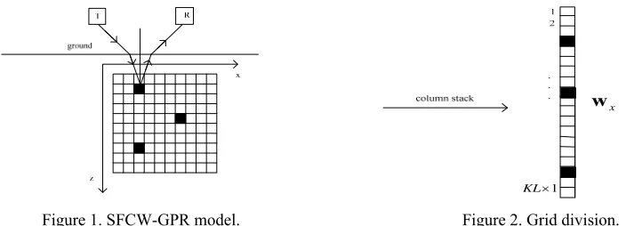
Figure 1. SFCW-GPR model. Figure 2. Grid division.

We assume the antenna measurement apertures areM , the scanning frequency of transmit antennas fromf₀ to f_N1in a scan period. Targets pare existed in the detection area. The complex echo signals can be obtained in each antenna measurement apertures as:

, 1

( ) P exp( 2 )

m n p n p m

p

f  j f 







s τ

(1) Where m1, 2M n, 1, 2N ,



p denote complex reflection coefficient of the

targetp,τ_{p m,} denote round-trip delay from antenna measurement apertures m to the target p. The figure1 can be converted into KL1 dimensions vector through column stack shown in figure

2 and denoted as w_x.The formula (1) can also be expressed as:

m m x

S B w ₍₂₎

Where dictionary matrixB_m N KL,S_m [ ( ), , (s₀ f₀  s_m f_N1)]T areN1dimensions frequency domain measurement vectors. s_m( )f_n are echo datas that the measurement aperture is mand the frequency is f_n. The jth column of dictionary matrix B_mcan be expressed as:

 

2 0m j, _{, ,} 2 N1m j,

T

j f j f

j e e

   _

 

 

  

m

B 

(3) Where j1,2KL,



m j, are round-trip delay from grid jto the measurement aperture m . The antennas measurement apertures are m , so all measurement datas can be combined the vectors

x

S , T

m

 

  T T T

x 1 2

S S ,S , ,S ,S_xNM1 . The corresponding dictionary matrix B_x can express as T

m

 

  T T T

x 1 2

B B ;B ; ;B .The relationship between Sx and reflection coefficient vectorswx as follows:

x  x x

S B w ₍₄₎ In general, reflection coefficient vectorsw_xare sparse, we randomly select the apertures Q1 from antennas measurement apertures m and the datasQ₂ from measurement datas N .Measurement matrixΨQ Q1 2NMandQ Q1 2NM ,the measurement vectors txcan be expressed as:

x x x x x

x ΨS ΨB w Θ w

t    _, Θx ΨBx, ΘxQ Q1 2KL (5)

MT-BCS Imaging Algorithm

R e( )

R e(

)

Im ( )

Im (

)

x x

x x

x x





























t

w

v

θ

t

w

Re( ) Im( )

Im( ) Re( )

x x

x

x x



 

  

 

Θ Θ

Φ

Θ Θ ₍₆₎

The formula(5) can be rewritten as:

x



x x



x

v

Φ θ

n

₍₇₎

( 1,..., )

x x  M

n _{are residual error vector corresponding to each task, each element in the residual}

error vector are following normal distribution of zero mean and variance reciprocal is



0_{. The}

density function of the compressed sampling vector vx under the parameters θxand



0can be

expressed[9]:

2

0 2

0

0

2

( ) ( ) e x p ( )

2

x x x x

N

x x

p v / θ ,









 



v  Φ θ

(8) For each element of θx is assumed to be Gauss prior distribution of zero mean:

2

1 ,

1

(

_x

)

K L

(

_{x j}

/ 0,

_j

)

j

p

N













v / α

(9)

,

x j



can be expressed the element j in the task x.



1, 2, , 2



T KL

  



α 

are a set parameters that

shared by all tasks. Hyper parameter

α

and residual error parameter



0 _{is assumed to follow} gamma distribution. According to Bayesian rule, posterior probability density function of x j, _are following multidimensional Gaussian distribution[10].

0 0

0

(

/

,

) (

/ )

(

/

, ,

)

(

/

,

)

(

/

,

) (

/ )

x x x

x x x x x

x x x x

p

p

p

N

d

p

p













v

θ

θ

α

θ

v α

θ

μ Σ

θ

v

θ

θ

α

(10)

x

μ

and Σx_{are the means and covariance respectively of coefficient vector for each task, they can}

be expressed as:

0

x





x x x

T

μ

Σ Φ v

1

0

(

)

x



x x





T



Σ

Φ Φ

A

₍₁₁₎

Where Adiag( , 1 2,2KL),Hyper parameter



can be obtained by fast relevance vector

machine[11], we obtain hyper parameter α, the coefficient vector θx can be solved by formula (11).

Simulation and Experimental Results

BCS （ ） crossrange cm （） dow nr ange cm

5 10 15 20 25 30 35 40 30 32 34 36 38 40 42 44 46 48 50 ₀ 0.1 0.2 0.3 0.4 0.5 0.6 0.7 0.8 0.9 1 BCS （ ） crossrange cm （） dow nr ange cm

5 10 15 20 25 30 35 40 30 32 34 36 38 40 42 44 46 48 50 ₀ 0.1 0.2 0.3 0.4 0.5 0.6 0.7 0.8 0.9 1 MT-BCS crossrange(cm) do w nr ange( cm )

5 10 15 20 25 30 35 40 30 32 34 36 38 40 42 44 46 48 50 0 0.1 0.2 0.3 0.4 0.5 0.6 0.7 0.8 0.9 1 MT-BCS crossrange(cm) dow nr an ge( cm )

5 10 15 20 25 30 35 40 30 32 34 36 38 40 42 44 46 48 50 ₀ 0.1 0.2 0.3 0.4 0.5 0.6 0.7 0.8 0.9 1

[image:4.612.86.523.68.159.2]

(a)Measurement ratio is 15% (b) Measurement ratio is 25% (a)Measurement ratio is15% (b) Measurement ratio is25% Figure 3. Reconstruction results of BCS. Figure 4. Reconstruction results of MT-BCS.

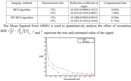
[image:4.612.80.512.252.518.2]

The experimental results show that BCS algorithm have more noise points and false targets. The reconstruction reflection coefficients and computational time of the two algorithms are given in table 1.

Table 1. Comparision of two algorithms. Imaging methods Measurement ratio Reflection coefficient of

target Computational time BCS algorithm 15%

25%

(0.1032,0.0906,0.1012) (0.1014,0.1018,0.0901)

0.842s 1.036s MT-BCS algorithm 15%

25%

(0.1008,0.0926,0.0914) (0.1021,0.1016,0.1018)

0.594s 0. 782s

The Mean Squared Error (MSE) is used to quantitatively analyze the effect of reconstruction.

2 2

ˆ

MSE f  f f

, f _and fˆ _{represent the true and estimated value of the signal.}

Figure 5. Comparision of reconstruction effects under different measurement ratio.

The results show that the MT-BCS algorithm can get better reconstruction performance than the BCS algorithm under the same observation data.

Summary

In the paper, the MT-BCS algorithm is be introduced. MT-BCS algorithm can exploit the statistical and structural characteristics of sparse signal, achieving reconstruction for many relevant signals at the same time. Experimental results have shown that the reconstruction performance of MT-BCS is better than the BCS algorithm under few observation data.

Acknowledgement

L2013069.

References

[1]L. Huang, P.Y. Wang, Q. Song, Stepped-Frequency Radar Imaging Algorithm Based on Compression Sensing, J. Applied Mechanics & Materials, 543-547(2014) 2609-2613.

[2]L.L. Qu, Q. Huang, G.Y. Fang, Stepped-frequency ground penetrating radar imaging algorithm based on compressed sensing. J. Systems Engineering & Electronics, 32(2)(2010) 295-297.

[3]D.L. Donoho, Compressed sensing, J. IEEE Transactions on Information Theory, 52(4)(2006) 1289-1306.

[4]Q. Wu, Y.D. Zhang, M.G. Amin, et al, Multi-Task Bayesian Compressive Sensing Exploiting Intra-Task Dependency, J. Signal Processing Letters IEEE, 22(4)(2015) 430-434.

[5]S.D. Babacan, R. Molina, A.K. Katsaggelos, Bayesian compressive sensing using Laplace priors, J. IEEE Transactions on Image Processing, 19(1)(2009) 53-63.

[6]S. Ji, D. Dunson, L. Carin, Multitask Compressive Sensing, J. IEEE Transactions on Signal Processing, 57(1)(2009) 92-106.

[7]F.Q. Wen, G. Zhang, B. De, Block Sparse Bayesian Learning Based Recovery Algorithm for Multitask Compressive Sensing, J. Acta Physica Sinica, 64(7)(2014) 70201-070201.

[8]Z. Zhang, B.D. Rao, Sparse Signal Recovery With Temporally Correlated Source Vectors Using Sparse Bayesian Learning. J. IEEE Journal of Selected Topics in Signal Processing, 5(5)(2011) 912-926.

[9]J. Yuan, L. Bo, K. Wang, et al, Adaptive spherical Gaussian kernel in sparse Bayesian learning framework for nonlinear regression. J. Expert Systems with Applications, 36(2)(2009) 3982-3989. [10]M.E. Tipping, A.C. Faul, Fast Marginal Likelihood Maximisation for Sparse Bayesian Model, C. International Workshop on Artificial Intelligence and Statistics. (2003) 3-6.