2017 2nd International Conference on Information Technology and Management Engineering (ITME 2017) ISBN: 978-1-60595-415-8
Track-before-Detect Algorithm Based on Gaussian Particle Cardinalized
Probability Hypothesis Density
Shuai WEI*, Xin-xi FENG and Quan Wang
Information and Navigation College of Air Force Engineering University, Xi’an 710077, China
*Corresponding author
Keywords: Track-before-detect (TBD), Cardinalized probability hypothesis density (CPHD), Gaussian particle filter (GPF), Infrared image.
Abstract. In unknown dim target number environment, a new track-before-detect (TBD) algorithm based on cardinalized probability hypothesis density (CPHD) filter is proposed. It can avoid the low tracking robustness and high computational amount. The Gaussian particle filter (GPF) approximated posterior densities as Gaussians, the mean and covariance of each Gaussian components in CPHD can be operated recursively by using particle filter, re-sampling is not required. Meanwhile, according to the actual TBD situation, updated the function for calculating particle weight. Simulation reveals that, compared with the conventional algorithm, the proposed is able to convey the cardinalized information more reliably, has lower computational time-consuming with a better tracking performance in multi-dim targets estimation.
Introduction
Technology of track-before-detect(TBD)[1] does not set the threshold for each scan, scaning data for energy accumulation to achieve dim target detection and tracking. The methods include Hough transform [2], dynamic programming [3] and particle filtering [4-6].
Recently, experts begin to solves the multi-target tracking problem by probability hypothesis density (PHD) filtering and cardinalized probability hypothesis density (CPHD) filtering [1-8]. In paper[9], the SMC-PHD filter combined with TBD to construct the state model and the sensor measurement model. In paper[10], CPHD-TBD filter is proposed to enhance the tracking robustness. The above two will result in high complexity. In paper[11], the Gaussian particle filter (GPF) is proposed to approximate the posterior distribution of the unknown state variables as Gaussian function. but isn’t good at number estimating[12].
This paper proposes a TBD algorithm (GPF-CPHD-TBD) based on Gaussian particle CPHD filtering. The filter is used to iterate the mean value and covariance of each Gaussian term. And the particle is only affected by its diffusion small region calculation likelihood. Combined with GPF updating particle weights, the simulation experiments are carried out. The proposed algorithm can effectively solve the multi-weak targets tracking problem in unknown number.
Multi-Target Dynamic Model and Measurement Model Target Dynamic Model
CPHD filter can be used in the model of non-Gaussian nonlinear motion and low signal-to- noise ratio of multi-small target motion. Assuming the target number at time k isNk, the state is
represented as T
, , , ,
p p p p p p
k =xk xk yk yk Ik
x ,
(
p, p) (
, p, p)
k k k k
x y x y and p k
I means position, velocity and energy
intensity target of p k
x . The dynamic function is:
(
)
+1= , , 1, 2,
p p
k fk k vk p= ⋅⋅⋅Nk
x x
Infrared Sensor Measurement Model
The measurement model describes the measurement data of a radar in a certain region in Cartesian coordinates. Set the radar observation area size isNx×Ny, whereNxandNydenote the number of units
in x-axis and y-axis directions respectively, each size of resolution unit
(
i j,)
is ∆ × ∆x y ,1, 2, x, 1, 2, y
i= ⋅ ⋅⋅N j= ⋅⋅ ⋅N .The measurement model at time k is the intensity of
(
i j,)
in known state, where: ( ) ( )( )
( ) ( ) ( ) ( ) , , 1 , , , , k Ni j p
k k k
i j p k
k
h n i j i j C z
n i j i j C
= + ∈ = ∉
∑
x ,(2)
where, n i jk
(
,)
is the measurement independent Gaussian white noise at the sensor resolution unit. Crepresents the target diffusion effect area, (i j,)
( )
pk k
h x is the signal strength expansion value of a
resolution unit in target p k
x , the spreading function of hkis approximated as:
( )
( )
(
) (
)
2 2
,
2exp 2
2 2
p p
p
x k y k
i j p x y k
k k
i x j y
I h π ∆ − + ∆ − ∆ ∆ ≈ − ∑ ∑
x (3)
where, Σ represents point spreading variance. The target likelihood function is approximately as:
(
)
(
( ))
( ) ( ) ( )(
)
( ) ( ) , , | |p p p p
i k j k i k j k
i j i j
p p
k k s n k k n k
i C j C i C j C
p z p+ z p z
∈ ∈ ∉ ∉
≈
∏ ∏
×∏ ∏
x x x x
x x (4)
where,
( )
p { , , 1, , 1, , },( )
pi k j k
C x = r−q⋅⋅⋅r− r r+ ⋅⋅ ⋅r+q C x =
{
s−q,⋅⋅⋅,s−1, ,s s+ ⋅⋅⋅1, ,s+q}
. q is the radius of diffusionregion of target p k
x , and (r,s) is the most influential image unit. The function of target SNR is:
2
/ 2 20 lg
p x yIk
SNR π
σ
∆ ∆ Σ
=
(5)
Normally, the SNR of infrared image below 10dB is regarded as a dim target, the target diffusion effect area less than 6×6 is regarded as a small target[12].
Gaussian Particle CPHD Filter in TBD Method Prediction
The cardinality distribution prediction is as:
( ) ( ) ( )
(
)
| 1 , 1 , ,
0
1
n
l j
l j
k k k j k s k s k
j l j
p n p n j C p l p p
∞ −
− Γ −
= =
=
∑
− ×∑
−(6)
where, pΓ,k
( )
⋅ indicates the cardinality distribution of birth target at the moment k, ps,k( )
⋅ meanstarget survival probability; and
( ) ! ! ! l j l C
j l j =
− . The intensity function is predicted to be:
( )
( )
( )
| 1 , | 1
k k s k k k
v − x =v − x +γ x (7)
( ) 1 ( )
(
( ) ( ))
, | 1 , 1 , | 1 , | 1
1
N ; ,
k J
i i i
s k k s k k s k k s k k
i
v p w
−
− − − −
=
=
∑
x x m P
(8)
( ) , ( )
(
( ) ( ))
, , ,
1
N ; ,
k J
i i i
k k k k
i
w γ
γ γ γ
γ = =
∑
The birthγk
( )
x ,i=1, 2,⋅⋅⋅,Jγ,k, ( )| 1 ( ),i i
k k k
w − =wγ ,
( ) ( ) ( ) ( )
| 1= , , | 1= ,
i i i i
k k− γk k k− γk
m m P P , ( ),
i k
wγ is the birth target Gaussian
weight. ( ) ( )
, , ,
i i
k k
γ γ
m P are the Gaussian mean and covariance of the newborn target separately.
Survival targetvs k k, | −1
( )
x ,i=1, 2, ,⋅⋅⋅ Jk−1, using Monte Carlo Gaussian particle sampling [9] can beobtained: ( )( ) ( ) ( )
(
)
( )( ) ( )( )(
)
1 ~ 1, 1 , , | 1~ | 1 1 , 1, 2, ,
i j i i i j i j
k k k s k k k k k
x− Ν m− P− x − f − x− j= ⋅⋅⋅M,where fk k|−1
( )
⋅ represents the target statetransition density function, ( )i1 k
w− is the weight of the i-th particle,
( ) ( )
, | 1, , | 1
i i
s k k− s k k−
m P are the mean and
covariance of survival target Gaussian term.
( ) ( )
| 1= , 1
i i
k k s k k
w − p w− (10)
( ) ( )( )
, | 1 , | 1
1
1 M
i i j
s k k s k k
j
m x
M
− −
=
=
∑
(11)( )
(
( ) ( )( ))
(
( ) ( )( ))
T, | 1 , | 1 , | 1 , | 1 , | 1
1
1 M
i i i j i i j
s k k s k k s k k s k k s k k
j
P x x
M
− − − − −
=
=
∑
m − m −(12)
Updating
The importance density functionπ
(
⋅|Z1:k−1,z)
is sampled at time k for particles( )( )i j k
x ,i=1, 2,⋅⋅⋅,Jk−1,
1, 2, ,
j= ⋅⋅⋅M,Zkis measurement set, wherez∈Zk. The cardinality distribution updating is as:
( ) ( ) ( )
0
| 1 | 1
0
| 1 | 1
,
, ,
k k k k k k
k
k k k k k k
w n p n
p n
w p
− −
− −
Ψ
=
Ψ
Ζ
Z
(13)
The intensity function is predicted to be:
( ) ( ) ( ) ( ) ( ) ( ) ( ) ( )
(
)
|1 1| 1 | 1
, 0 | 1
1 | 1 | 1
, ,
1 ; ;
, ,
k k
k J
k k k k k k i i i
k D k k k k k k
z Z i k k k k k k
w p
v p v w z
w p − − − − ∈ = − −
Ψ
= − + Ν
Ψ ∑ ∑
Z
x x z x m p
Z (14) [ ]( ) ( )
(
)
(
)
(
)
( ) ( )(
)
min , ,k , 0 1 , ! , 1,n j u z n
D
u n
k K k j u j u j k
j
p
w n j p j P e w
w − +
+ +
=
−
Ψ Z =
∑
Z− Z− × Ξ Z(15) ( ) ( ) ( ) ( ) , , 0 ! , , , ! 1 0 n j j j j n
P x x dx e
n j
j ζ
ζ
α β α β ⊆ = ∈
≠ = − = = = ∑ ∏
∫ Z S Z S S
(16)
Considering the TBD directly to the original image processing, the target detection probabilities pD,k are approximately 1[10], and the particle likelihood is only related to its influence region C.
Assuming a new measurement at the moment k, when a particle is subjected to likelihood calculation, the whole measurement set is divided into:
(
| 1)
(
| 1)
nn p p
p k =Vp k k− V k k−
Z x ∪ x
(17) The combined likelihood ratio of the particle to the measurement is:
( )
(
)
( ) ( ) ( )(
)
( ) ( ) ( )( |1) |1
, , ,
| 1 2
2
| exp
2
p p
i k k j k k
i j i j i j
k k k
p p k k k k
i C x j C x
h h g V σ − − − ∈ ∈ − =
∏
∏
Zx
(18)
When ( )i j, n
p k ∈V
Z , there is
(
| p| 1)
0k k k
g z x − = , a particle | 1 p k k−
x is corresponding to the likelihood domain p k
V ,
( )( ) ( ) ( )
(
)
( ) ( )(
(
)
)
( ) | 1 | 1, | 1
1 | 1, , ! , 1, p p k k k k
i j i k
k k k p
k
j k k
n
K k j n k k
g V M
w w j n
z
e w V
j p j P p
w κ κ − − − = = Ξ − − × x Z Z , (19)
where, κk is clutter intensity function, pK k, is clutter cardinality distribution function, Z is
calculating likelihood measurement with a particleXk kp| −1, there is:
(
)
( )
( )
T 1,
, p k p : p
k k k k k k
k
w V w g V V
z
κ κ
Ξ = ∈
Z
(20)
( ) ( )
( )
( )(
)
( )(
)
|1 |1
T T
1 1
| 1 | 1, | 1 , | | 1 , | | 1
k k k k
J p p p J
k k k k k k k k k k k k k k k k
w w w − g V g V g V −
− − − − −
= ⋅⋅⋅ = ⋅⋅⋅
x x (21)
The updated Gaussian weights, mean and covariance are:
( ) ( )( )
1 M
i i j
k k j w w = =
∑
(22) ( )( )
( )( ) ( )( ) ( ) 1 Mi j i j
k k
i p j
k k i
k w x V w = =
∑
m (23) ( ) ( )( ) ( )( )
( )( )(
)
( )( )
( )( )(
)
( ) T 1 Mi j i p i j i p i j
k k k k k k k
i j
k i
k
w V x V x
w =
− −
=
∑ m m
p
(24)
Pruning and Merging
To avoid the infinite number growth, we need to adopt pruning and merging algorithm[13], keep the Gaussian term with large weight and set the threshold T. Delete the Gaussian term whose weight is less than T and merge the similar Gaussian term whose distance is less than U.
Estimate Target States
We adopt the method of Maximum A Posterior (MAP) for GPF-CPHD-TBD algorithm to estimate the state and number of targets. Choose the mean of Gaussian term which conforms to ( )i
k
w > 0.5 as the target state, and estimate the number of targets then, the expression is as follows:
( )
arg max
k k
N = p n
(25)
Simulation Experiments and Analysis
To verify the feasibility and effectiveness of the proposed algorithm, we make a comparison between the proposed algorithm and SMC-CPHD-TBD, GPF-PHD-TBD algorithms.
Experimental Parameters
The state function isXk+1=FXk+Rk, Rkis white Gaussian noise. The target detection probability is 1,
the survival probability is 0.99, the birth probability is 0.1, the disappearance probability is 0.01, and the derivation probability is 0. The whole process is last for 60 frames, the interval frame is 1 second, the pixel resolution unit is ∆x=∆y=1 , the image size is 80×80 sequence,
(
)
=0.7, U 18, 22
∑ Ι ∈ ,T=10-5, U=4. There are three targets in airspace, their initial states are as
follow: [ ]T [ ]T [ ]T
1= 5, 0.15, 6.4, 0.1, 20 , 2= 7.8, 0.12,1, 0.1, 20 , 3= 2, 0.1,8.2, 0.12, 20 .
X X X Target 1 appears throughout
Figure 1. Infrared measurement images.
[image:5.612.82.529.417.511.2]Simulation and Analysis
Figure 1 shows the infrared measurement images at t=5,18,38,55s under SNR=5.7dB respectively. The Optimal Sub-pattern Allocation (OSPA) distance[15] is used as the criterion of evaluation, setting the parameter c = 5, p = 2. Assume that the new target location is unknown. We assume the different SNR (10, 7.3, 5.7dB) environment for simulation, The number of particles per frame is 2000, and the Monte Carlo simulation is 100 times. The results are as follows.
(a) OSPA cardinalized distance in SNR10
(b) OSPA cardinalized distance in SNR7.3
(c) OSPA cardinalized distance in SNR 5.7
Figure 2. Three filter simulation comparison on OSPA cardinalized distance in different SNR environments.
Figure 2 reflects the overall performance of the target number estimation. The OSPA of GPF-CPHD-TBD is always low, and the tracking performance is always good even in the worse SNR of 5.7dB, indicating that the proposed algorithm can estimate the number of targets accurately.
[image:5.612.83.530.586.663.2](a) OSPA location distance in SNR 10 (b) OSPA location distance in SNR 7.3 (c) OSPA location distance in SNR 5.7 Figure 3. Three filter simulation comparison on OSPA location distance in different SNR environments.
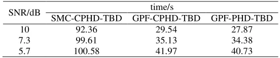
Table 1. Three filters comparison on time running in different clutter situations.
SNR/dB time/s
SMC-CPHD-TBD GPF-CPHD-TBD GPF-PHD-TBD
10 92.36 29.54 27.87
7.3 99.61 35.13 34.38
5.7 100.58 41.97 40.73
The GPF-CPHD-TBD is about 36% of time-consuming by the SMC-CPHD-TBD because each Gaussian only be assigned a small amount of particles to achieved good performance. Although GPF-CPHD-TBD takes longer time, it can estimate target much more stably than the others.
Conclusion
We propose a multi-target TBD tracking algorithm based on Gaussian particle CPHD, which updates the mean and covariance of the target state iteratively without re-sampling. The proposed can effectively reduce the computational complexity, improve the computational efficiency, the accuracy and stability of dim target number and state estimation, to solve the problem of unknown target detection and tracking in low SNR.
Acknowledgements
This work was partly supported by the National Natural Science Foundation of China (61571458).
References
[1]Buzzi S, Lops Ma, Venturino L. Track-before-detect procedures in a multi-target environment[J]. IEEE Trans. on Aerospace and Electronic Systems, 2008, 44(3): 1135-1150.
[2]Moyer L R, Spak J, Lamanna P. A multidimensional Hough transform based track-before-detect technique for detecting weak targets in strong clutter backgrounds[J]. IEEE Trans. on Aerospace and Electronic Systems, 2011, 47(4): 3062-3068.
[3]Deng X, Bi R, Liu H. Threshold setting of track-before-detect based on dynamic programming for radar target detection [C]. Proc. of the IET International Radar Conference, 2003: 1-4.
[4]Salmond D J, Birch H. A particle filter for tract-before-detect[C]. Proc American Control Conference, 2001:3375-3760.
[5]Boers Y, Driessen H, Torstenson J, et al. Track-before-detect algorithm for tracking extended targets [J]. IEEE Proc. Radar Sonar Navig, 2006,153(4): 345 -351.
[6]Zhao F, Liu H Z, Zhang Z Y. Infrared ship tracking based on improved multi-features fusion based mean-shift[J]. System Engineering and Electronics, 2014, 36(2): 205- 213.
[7]Mahler R. PHD Filters of Higher Order in Target Number[J]. IEEE Trans. on Aerospace and Electronic Systems, 2007, 43(3): 1523-1543.
[8]Vo B N, Singh S, Doucet A. Sequential Monte Carlo methods for multi-target filtering with random finite sets[J], IEEE Trans. on Aerospace and Electronic Systems, 2005, 41(4): 1224-1245.
[9]Punithakmar K, Kirubarajan T, Sinha A. A sequential Monte Carlo probability hypothesis density algorithm for multi-target track-before- detect[C]. Proc. of the Signal Data Processing Small Target, 2005, 5913: 1-8.
[11]Jayesh H.K, Petar M.D. Gaussian particle filtering [J]. IEEE Trans. on Aerospace and Electronic Systems, 2001: 429-432.
[12]Li C Y, Cao X N, Liao L X, Jiang Z. Track-before-detect using Gaussian particle probability hypothesis density[J]. System Engineering and Electronics, 2015, 37(4): 740- 745.
[13]Vo B N, Ma W K. The Gaussian mixture probability hypothesis density filter. IEEE Trans on Signal Processing, 2006, 54(11):4091-4104.
[14]Ou Y C, Ji H B, Zhang J G. Improved CPHD filter for multi-target tracking[J]. Journal of Electronics and Information Technology, 2010, 32(9): 2112-2117.