2017 2nd International Conference on Computational Modeling, Simulation and Applied Mathematics (CMSAM 2017) ISBN: 978-1-60595-499-8
Non-Rigidity Objects Tracking in Dynamic Scenes Using Particle Filter
Xiao-xue SUN
*No.77, Hanlin Road, Economic and Technological Development District, Jilin, China
*Corresponding author
Keywords: Object tracking, Bayesian estimation, Particle filter, Color histogram.
Abstract. Particle Filter (PF) method is an efficient tool for non-rigidity objects tracking. The paper presents a Bayesian-based PF method for objects tracking in dynamic scenes. The paper discusses the Bayesian estimation algorithm and the PF process. The color histograms are used as the measurement to obtain the optimized posteriori probabilities by comparing the histogram of the particles’ rectangles in the sequence images with the reference histogram. The robust mean technique is applied to ascertain the objects’ positions. The author performed single object and multi-objects tracking in the experiments. In this paper, I compared the PF method with the mean-shift algorithm, and the result shows that the PF method is more efficient.
Introduction
Non-rigidity object tracking in the sequence images is the problem of motion estimation. The characteristic of the estimation is the ruleless motion and difficult to describe. The frame difference method could be used in the static scenes tracking but not in the dynamic scenes because the frame difference method could not get the results. The method base on statistics should be employed in this case.
The methods based on the statistics always using the theory of Markov Random Field (MRF) to estimate the object model in the image sequence [1, 2]. The Bayesian Filter (BF), Dynamic Monte Carlo (DMC) theory, Kalman Filter (KF), Sequential Monte Carlo (SMC) method and so on, are included in the theory framework. The Sequence Monte Carlo method is also named Particle Filter (PF) [3-5]. The Mean-Shift is also an important and efficient method.
The KF algorithm estimates the non-linear motion of the object approximately by parameter optimization [6]. The main short point of them is the strict request for filter error and measurement error. If the errors could not fit the request, the tracking would be failed completely. The PF method is used in the dynamic scenes for object tracking using the object probability obtained according to the object characters [7,8]. So, the tracking would not be affected by the similar objects in the scenes. The PF is non-parameter MC simulation method. It gets the optimization estimation by iterative BF. The Mean-Shift algorithm could also track the object in the dynamic scenes. But for the multi object tracking, the objects in the image sequence will be affected by each other that make the tracking result fail. Using the algorithm proposed in this paper, the effect from the other objects would be avoided by weight updating and particle resample.
The Bayesian Estimation is discussed in the second part of this paper. The PF theory based on the BF was depicted in the third part in this paper. In the fourth part, we used the histogram of the object as the measurement to perform the PF tracking procedure. The fifth part of the paper is the experiments. In this part, the image sequence “tennis” and the image sequence shoot in the real scene. The image sequence “hockey” is used to compare with the Mean-Shift algorithm so that to prove the efficiency of the method proposed.
Bayesian Estimation
) , ( ) , ( 1 k k k k k k k k v x h y w x f x
. (1) in which, xk is the state vector in the n dimensions space Rn. wk is the noise whose mean is 0. vk is the measurement noise. If the measurement yk is given (k is the parameter of time), and it means that the current image is the kth frame), the aim is to estimate the state ofxk. The optimization estimation of the minimum variance can be expressed as
] | [ k 1k
k Ex Y
X
. (2) in which, Y1k [y1,y2,...,yk] is the measurement image sequence till the time k. The optimization
estimation needs the posteriori probability density p(xk|Y1k), and the posteriori probability density
could give us minimum variance error and many optimization estimation results [9]. The method that got the posteriori probability density was Bayesian algorithm in principle and the state probability density will be got according to the following formula
k k k k k k k k k k k dx x y p Y x p x y p Y x p Y x p ) | ( ) | ( ) | ( ) | ( ) | ( 1 1 1 1 0. (3) In the Bayesian estimation, p(xk|Y1k1) could be expressed as
P(xk|xk1)p(xk1|Y1k1)dxk1 though theupdating procedure and the Bayesian estimation could be got by the combination of p(xk|Y1k1) and
the formula (3). In the KF, the main method is also Bayesian estimation. But in KF, the state formula and the measurement formula are all assumed to be linear and the noise is assumed as Gaussian noise. So, it can not solve the non-linear problems as the object motion estimation. The PF algorithm uses the sampling method to simulate the posteriori probability density.
Particle Filter Theory
The PF algorithm expresses the posteriori probability p(xk|Y1k) by a set of particles with weights. For
example, there is a set of particles {x1k,...,xkn} sampled from xk at time k, and there is a set of weights
} ,...,
{s1k skn according to the particles and the weights based on the unitary rule, 1 1
n i i ks , in every step.
In the first step, n ski
1
. If the whole state vector can be expressed as Xk {x1,x2,...,xk}, the posteriori
probability can be shown as the combination of the particles and weights. The particle can be regarded as the swatch sampled from the weightiness distributed formula. The posteriori probability can be got through an iterative procedure as follows [10].
Firstly, we assumed that p(xk1|Y1k1) is the posteriori probability at time k-1 and it was already be
obtained. The particles set is {x1k1,...,xnk1} and the weights set is {s1k1,...,snk1}, so
n i i k k i k kk Y s x x
x p 1 1 1 1 1 1
1| ) ( )
(
. (4) in which () is Kronecker Delta function. According to the description above, p(xk|Y1k1) can be
obtained by ( 1| 11) k
k Y
x
p , that is
1 1 1 1 1 11 ) ( | ) ( | )
|
(xk Yk p xk xk pxk Yk dxk
p
. (5) The recursion procedure defines the current state posteriori probability as the function of the prior probability and the current measurement data. The model of state space is realized by defining the state transform probability p(xk|xk1) and measurement probability p(yk|xk). The p(xk|xk1) is
After this, we can get the measurement yk of the time k. As the formula (3), the prior distribution
) |
( 11
k
k Y
x
p can be got by model updating. In the process, the weights set can be obtained by importance sampling method and the weight of the ith particle is
) | ( ) | ( 1 1 k i k k i k i k Y X q Y X p s
. (6) The importance distribution function can be segmented as
) | ( ) , | ( ) |
(Xk Y1k q xk Xk1 Y1k q Xk1 Y1k1
q . (7)
We can get the particle i k
x through q(xk|Xk1,Y1k) and get the particle set Xki1 through q(Xk1|Y1k1).
If q(xk|Xk1,Y1k)q(xk|xk1,yk), that is the importance distribution function depend on the current
measurement yk and the last state xk1. So, according to the weight formula (6), we get the weight updating formula ) , | ( ) | ( ) | ( ) | ( ) | ( 1 1 1 1 1 k i k i k i k i k i k k i k k i k k i k i k y x x q x x p x y p s Y X q Y X p s
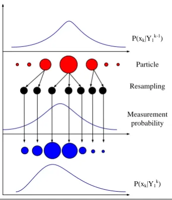
. (8) At last, the particle retrogression in the performing procedure should be noticed. After some iterative steps, the weights of the particles become very small except one particle and this makes the calculating time wasted in the useless particles updating. The case described above is called particle retrogression. To solve this problem, we can take two methods including choosing the importance distribution functionand resample.
The best importance distribution function q(xik|xki1,yk) can be chosen by the following formula
) , | ( ) , |
( ki 1 k k ik 1 k i
k x y px x y
x
q ( | )
) | ( ) , | ( 1 1 1 i k k i k k i k k k x y p x x p x x y p
. (9) Only ifp(xk|xki1,yk)p(xk,xik1), according to formula (8), we can get that
) |
( 1
1 k ki i
k i
k s p y x
s . (10) The purpose of resample is removing the particles with small weights. We sampled the measurement according to the weights sik i1,2,...,n and get the new particles, so that to increase the
particles with big weight values. The particle weights should be united by n ski
1 .
P(xk|Y1k-1)
Particle
Resampling
Measurement probability
[image:3.595.210.384.561.764.2]P(xk|Y1k)
Particle Filter in the Object Tracking
In the color image sequence object tracking, we can set the state vector as
T y x i yk i xk i
k c c H H
x [ , , , ]
. (11) This vector is the position of the particle. Hx and Hyare the width and height of the rectangle around the particle. We don’t regard the whole image yk but the color image histogram hk as the measurement and the calculation is performed in the image field according to the state vector i
k x . The Gaussian probability density is used as the likelihood function of the color image histogram and the function is defined as following
} 2
) ( exp{ 2
1 ) , 0 ; ( ) | (
2 2
2 2
ki
i k i
k k
D D
N x h
p
. (12) In the formula (12), i
k
D is the distance, expressed by the state vector xik, between the histogram hk
and the reference object histogram *
q in the current image. In the formula (12), is the variance of the Gaussian density. The Bhattachary parameter is defined as [h,q]
h(u)q(u)du should becalculated to get i k
D . The histogram should be calculated in the rectangle u according to the state
vector. So, the histograms should be defined as { ( )} 1,2,3,..., . m u u h
h and q{q(u)}u1,2,3,...,m., and the parameter is
m
u
u u
q h q
h
1
) ( ) (
] , [
. (13) The distributions are more close to each other with the increasing of the parameter . If the 1, it is shown that the two histograms are same. We defined the distance between the two distributions as
] , [
1 hq
Dki . (14) According to formula (12) and (14), the Bayesian posteriori probability will be got based on the color histogram.
In the next step, we should find the position of the object according to the distribution of the particles. Three methods are regularly used including particle mean, the best particle and the robust mean technique. In the particle mean method, we calculate the mean of the particles at last. In the best particle method, we choose the particle with the biggest weight to express the position of the object. In the last method, we use the particles in a small window around the best particle. After analysing, the particle mean method should not be chosen for the case of multi objects. And the best particle method should not be used for the discrete error. The calculation account is big in robust mean technique. In this paper, we use the robust mean technique.
Experiments
(a) (b) (c)
[image:5.595.131.465.68.265.2]
(d) (e) (f)
Figure 2. The single object tracking of the basketball image sequence.
The second experiment uses the standard image sequence named “hockey”. The method proposed in this paper is compared with the Mean-Shift algorithm. The tracking is done for the 81st to the 170th frame of the sequence. The tracking results of the Mean-Shift are shown in Figure 3 and the results of the proposed method are shown in Figure 4. In the images, the first object is marked by the blue rectangle, the second object is marked by the green rectangle. The results are generally same in the first part of the sequence tracking. In the following tracking, object 1 and object 2 does not tough each other (shown in image (b) and (c) of Figure 3. and Figure 4). From image (d), the object 1 and 2 tough each other and the result are natural in the two tracking sequence. From the 154th frame, in the Mean-Shift result, the object 2 is affected by the object 1 and in the 160th frame, the object 2 is lost. But in the proposed method tracking, the object 2 tracking is successful in the whole procedure.
Conclusions
Statistical algorithm is a very important way for image modeling in image segmentation and reversion especially the EM and the MRF method. But the classical EM method did not introduce the spatial information to the image model. The classical MRF potential functions always do not involve the relationships of pixel intensities and the distances between pixels. So, for image segmentation, the results were negatively affected by these factors. To overcome these problems, a novel potential function, which involved the pixel intensity and distance values, is introduced to the traditional MRF image model. Then, the segmentation problem is transformed to MAP procedure and the ICM method is employed to obtain the MAP solution. The experiment results prove that the algorithm proposed in this paper is an efficient method for images segmentation.
(a) (b) (c) (d)
(e) (f) (g) (h)
[image:5.595.83.512.589.766.2]
(a) (b) (c) (d)
[image:6.595.84.516.78.255.2]
(e) (f) (g) (h)
Figure 4. Tracking results of “hockey” using proposed method. (a) The 81st frame; The 112th frame; The 136th frame; The 146th frame; The 151st frame; The 154th frame; The 160th frame; The 170th frame.
References
[1] J. Vermaak, P. Perez, M. Gangnet, and A. Blake. Towards improved observation models for visual tracking: selective adaptation. In Proc. Europ. Conf. Computer Vision, Copenhagen, Denmark, May 2002.
[2] D. Comaniciu, V.Ramesh, and P. Meer. Real-time tracking of non-rigid objects using mean shift[J]. In Proc. IEEE Conf. Comp. Pattern Recog. June 2003: 142-149.
[3] B. Ristic, S. Arulampalam, and N. Gordon, Beyond the Kalman filter: Particle filters for tracking applications, Artech House, 2004: 154-157.
[4] K. Nummiaro, E. Kollor-Meier, and L. Van-Gool. Color-Based Particle Filter[J]. Image and Vision Computing. 2003 vol 21: 99-110.
[5] P. Perez, C. Hue, J. Vermaak, and M. Gangnet. Color-Based Probabilistic Tracking. A. Heyden et al. (Eds.): ECCV 2002, LNCS 2350, pp. 661–675, 2002.
[6] Arulampalam Sanjeev, Maskell Simon, Gordon Neil, Clapp Tim. A tutorial on particle filters for online non-linear non-Gaussian Bayesian tracking. IEEE Transactions on Signal Processing, 2002, 50 (2): 174-188.
[7] Leung Chung-Chu, Chen Wu-Fan. Brain tumor boundary detection in MR image with generalized fuzzy operator. Proceedings of IEEE ICIP Conference, Barcelona, Spain, 2003: 14-17.
[8] Geman, S., Geman, D, Stochastic relaxation, Gibbs distributions, and the Bayesian restoration of images. IEEE Trans. on Pattern Analysis and Machine Intelligence, vol.6, pp. 721-741, 1984.
[9] Won Kim, Choon Young Lee, Ju Jang Lee. Tracking moving object using Snake’s jump based on image flow. Mechatronics, 2001, (11): 119-216.