http://dx.doi.org/10.4236/jep.2013.411A008
Effects of Sea Level Variation on Biological and Chemical
Concentrations in a Coastal Upwelling Ecosystem
Marilia M. F. de Oliveira1*, Gilberto C. Pereira1, Jorge L. F. de Oliveira2, Nelson F. F. Ebecken1
1Civil Engineering Program, Federal University of Rio de Janeiro-UFRJ, Center of Technology, Fundão Island, Rio de Janeiro, Brazil; 2Geography Postgraduate Program, Fluminense Federal University-UFF, Geoscience Institute, Niterói, Brazil.
Email: *marilia@coc.ufrj.br
Received September 8th, 2013; revised October 8th, 2013; accepted November 8th, 2013
Copyright © 2013 Marilia M. F. de Oliveira et al. This is an open access article distributed under the Creative Commons Attribution License, which permits unrestricted use, distribution, and reproduction in any medium, provided the original work is properly cited.
ABSTRACT
Oscillations in sea level due to meteorological forces related to wind and pressure affect the regular tides and modify the sea level conditions, mainly in restricted waters such as bays. Investigations surrounding these variations and the biological and chemical response are important for monitoring coastal regions mainly where upwelling shelf systems occur. A spatial and temporal database from Quick Scatterometer satellite vector wind, surface stations from the South-east coast of Brazil and surface seawater data collected in Anjos Bay, Arraial do Cabo city, northSouth-east of Rio de Janeiro State were used to investigate the meteorological influences in the variability of the dissolved oxygen, nutrients, mero-plankton larvae and chlorophyll-a concentrations. Multivariate statistical approaches such as Principal Component Analysis (PCA) and Clustering Analysis (CA) were applied to verify spatial and temporal variances. A correlation ma-trix was also verified for different water masses in order to identify the relationship between the above parameters. A seasonal variability of the meteorological residual presents a well-defined pattern with maximum peaks in au-tumn/winter and minimum during spring/summer with negative values, period of occurrence of upwelling in this region. This lowering of the sea level is in accordance with the increasing of nutrients and meroplankton larvae for the same period. CA showed six groups and an importance of the zonal and meridional wind variability, including these variables in a single cluster. PCA retained eight components, explaining 64.10% of the total variance of data set. Some clusters and loadings have the same variables, showing the importance of the sea-air interaction.
Keywords: Meroplankton Larvae; Nutrient Concentrations; Coastal Waters; Brazilian Upwelling
1. Introduction
The upwelling shelf systems as reservoirs for biological and chemical concentrations depend as much on the scales and rates of phytoplankton new production as on the dynamical processes that govern heterogeneity of particle sedimentation within the shelf [1]. Tropical seas occurs greater light penetration in the water column, varying little throughout the year which makes it an op- timum condition for phytoplankton primary production and so, increasing the concentration of chlorophyll a.
In coastal regions subject to the influence of coastal upwelling, phytoplankton production can be greatly af- fected locally. The transport to the surface of deep water cooler, nutrient rich favors the occurrence of major phy- toplankton production peaks that can determine the oc-
currence of maximum abundance of zooplankton popula- tions [2]. Internal tides and coastal upwelling have im- portant roles in marine ecosystems due to the mixing of water masses with potential redistribution of heat, salt and nutrients to the biological system. There are numer- ous mechanisms whereby tides might influence shoreline biological and chemical concentrations. Flooding tides can dilute near shore sources and reduce these concentra- tions. Ebbing tides drain the water from land to sea and spring tides provide a hydrologic connection between the sea and biological and chemical sources at the high water line and upper reaches of the tidal prism in tidal wetlands and subterranean estuaries within the beach aquifer [3].
A flow pattern observed in continental shelf and slope associated with tidal currents is highly modified by fac- tors such as topology of coastline, background bathym- etry and climatic conditions of the region. These currents
can generate resuspension of sediments and nutrients from the bottom, increasing the mixing layer. Barotropic and baroclinic tides can cause a mixing in the water col- umn, leading an important impact on biological produc- tion due to the upward flow of nutrients from the layers below the euphotic zone [4].
Coastal regions are areas with high rates of productiv- ity in the marine environment, and are the areas that suf- fer most from the impacts of human activities on fish stocks and the pollution from the large coastal urban centers. Human activities such as fishing, shipping and recreation are also centered near the shorelines, where knowledge of the tidal movement is necessary. These coastal regions are areas where tidal ranges are most evident and can, associated with elevated wave energy, cause coastal erosion. Hydrographic mesoscale structures in the South Atlantic subtropical ocean near the Brazilian coastline show a high variability in a environmental con- ditions, with physical and biological characteristics ex- tremely relevant with mechanisms of ocean-atmosphere (OA) interactions [5]. The upper ocean plays a funda- mental role in building a structure of both wind-driven and thermohaline circulation. Large-scale meteo-ocean- ography patterns are in accordance with the OA interac- tions through the South Atlantic subtropical high-pres- sure system, a predominant air mass above the central region of the South Atlantic Ocean basin, centered near 30˚ latitude that induces the currents of upper ocean due to the wind-driven forces [6]. This air mass modulates the zonal wind field and when easterly winds are domi- nant in the southeast coast of Brazil, high atmospheric pressure enhances the inflow of Atlantic waters through the Arraial do Cabo region. The water inflow leads to occurrence of coastal upwelling due to the anticyclonic gyre moving Tropical Waters (TW) off the coast fol- lowed by the up-flow of the deeper South Atlantic Cen- tral Water (SACW) mass, with a decrease in sea surface temperature and a maximum of surface nutrient concen- trations located in the coastal area. This pattern is pre- dominant in spring-summer period. On the other hand, in autumn-winter period, when southwesterly winds prevail, lower atmospheric pressure increases the flow parallel to the coastline and the oceanographic and biological struc- tures are different. These physical alterations also induce changes in the distribution of these variables.
Oscillations in sea level due to meteorological driving forces related to wind and pressure occur at different scales and frequencies in all coastal regions. Interactions between meteorological and oceanic variables affect the regular tides and modify the sea level conditions, mainly in restricted waters such as bays. The patterns of tidal waves on the continental shelf are scaled down, being strongly influenced by Kelvin wave dynamics and by basin resonances [7]. Tides on the continental shelf are
predicted using the harmonic analysis method which is based in tidal variations represented by N harmonic con- stituents. These constituents can then be used to provide reliable predictions for future tides at the respective point [8]. Predictions for reference stations are prepared from the astronomical arguments using local constituents de- termined by previous analysis and do not take into ac- count meteorological influences. Thus, the observed and predicted values of the sea level variations are normally different. Storms are the main cause of these sea level variations known as storm surge and the action of wind stresses on the surface water is the principal factor in- volved in the generation and modification of the sea level height [7,9,10]. The tendency for surge peaks that occur most often on the rising tide in UK North Sea coastline, using numerical models was confirmed by [11]. They concluded that this pattern occurs independently of the phase between tide and surge. The models made it possi- ble to separate the contribution to interaction from shal- low water and bottom friction. [12], see also [13] used an analytical model to show that the shallow water effect becomes dominant for great tidal amplitudes in depths of 10 m or less.
The variability of productivity in upwelling shelf re- gions must consider the need for a better understanding of the mean distributions and variability of nutrients, as well as the physical—biological coupling, in these re- gions. Upwelling systems are characterized by the ascen- sion of cold and rich in nutrients water that disturb eco- system dynamics and increases the environmental het- erogeneity [14]. Then, the knowledge about the sea level height variations in shelf regions is very important not only for marine services but also for designing and con- structing onshore structures, protection of coastal regions, and mainly for monitoring the changes in marine ecosys- tems [15].
This study is part of the research developed by the Federal University of Rio de Janeiro—Civil Engineering Program in remote monitoring systems of environmental impacts in coastal regions in order to develop trophic dynamic models to be used in the National Plan and Re- gional Coastal Management or in any other aquatic sys- tem. To continue the study of biological and chemical distribution and meteo-oceanography patterns [16], we have also verified the relations between them and tidal influence in the Arraial do Cabo region. This place is known for its active wind induced shelf upwelling [17]. Seasonal variability of the South Atlantic high pressure system is associated with the occurrence of this pheno- menon.
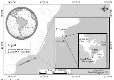
tic high-pressure system and is situated on the southeast coast of Brazil near Arraial do Cabo city, (Figure 1). small spatial scale [19]. Moreover this place is very at-
tractive for the tourist and recreational activities, contrib- uting to the local economy, but human activities are sig- nificantly affecting the coastal ecosystem [20]. The in- fluences of meteorological patterns in the sea level re- sponse at Arraial do Cabo was verified using the Quick Scatterometer satellite vector wind over the South Atlan- tic Ocean near the coast of the study area, surface sta- tions and seawater harvest sample, applying statistical tools such as multivariate analysis.
2.2. Climatological Description of the Study Area
This region is influenced by persistent high pressure over the South Atlantic Ocean that enhances northeast flow across the area. This circulation is periodically disturbed by the passage of frontal systems caused by migrating anticyclones that move from the southwest across the northeast in the southeast coast of Brazil.
The aim of this study is to investigate the influences of the sea level variations in the biological and chemical responses at Arraial do Cabo due to meteorological forc- ing, considering the main water masses in the southeast- ern Brazilian shelf.
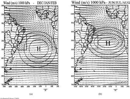
During the summer (Figure 2(a)), the subtropical high, over the continent, becomes weaker than winter (Figure 2(b)), moving southerly and on its western side the winds blow northeasterly towards the southeastern coast of South America and they are more intense in the south- eastern coast of Brazil. Therefore, in the north region of the Brazil Malvinas Confluence (BMC), at 38˚ - 40˚S, there is an intensification of the northerly winds and a weakening of the southwesterly winds which is difficult for the track of the cold fronts that reach the south and southeast coast of Brazil [21]. This seasonal variability is one of the most important factors related to the occur- rence of upwelling in the region of Arraial do Cabo, where the winds blow along the coastline from north to south push the surface waters offshore on summer peri- ods [18].
2. Material and Methods
2.1. Study AreaIn order to investigate the sea level dynamic in Arraial do Cabo and its influence in the variability of the studied variables, we verified the spatial and temporal meteoro- logical systems related to the sea level variations. This research is a continuity of [16], in which we used the same study area with the local points from satellite data, surface weather station, tide gauge station and sample water harvest in Anjos Bay.
This study area is under influence by the South Atlan- The mean surface circulation of the South Atlantic
[image:3.595.111.488.429.695.2](Adapted from [16]).
(a) (b)
[image:4.595.83.508.83.408.2](Adapted from [16]).
Figure 2. Surface wind-flow pattern with a scheme of the South Atlantic high-pressure system for summer (a) and for winter (b). The circles represent the isobars and the positions of the high centers moving slightly during the year; the squared shows the winds blowing over the study area; BMC Brazil Malvinas Confluence region.
Ocean is dominated by a closed system known as the South Atlantic subtropical gyre that is composed of sev- eral ocean currents and on the western boundary of this gyre it has the Brazil Current (BC) [22]. Thus, the South- west Brazilian coastline is characterized by the presence of the BC, a warm current of the South Atlantic that goes away inshore from the northern Brazil over a continental shelf toward the south, carrying the TW from the vicinity of the Equator [23]. This current makes this region oligo-trophic; therefore, in some areas occur a seasonal wind-driven upwelling of cold, nutrient-rich SACW mass, benefiting on biological productivity. In Arraial do Cabo, the positioning of the Cabo Frio island (23˚S, 42˚W) forms the small (45 Km2) and narrow (~10 m deep)
An-jos Bay (Figure 1).
The latitudinal position of the BC is characterized by a seasonal variation. It means that, on average during the austral summer, the BC extends more southwards. The opposite occurs in winter and BC extends more north- wards [22]. The transport of BC that follows the curve of annual variation of wind shear over the subtropical basin with a maximum during the summer (Figure 3) and minimum during the winter (Figure 4) was suggested by
[24].
The interest in monitoring environmental impacts in this coastal region is because it can be considered yet a pristine area and the hydrologic conditions are strongly influenced by the wind pattern that influences the distri- bution of water masses. Winds that blowing from north- eastern and the Earth’s rotation, result in a shunting of the nutrient-depleted surface TW of BC to offshore fol- lowed by the up-flow of the deeper (~300 meters) and nutrient-rich of SACW mass [20]. Upwelling events and inorganic nutrients are then supplied to euphotic zone by the exchange of water between nutrient-depleted surface water and nutrient-rich deeper water. When the inverse wind pattern occurs, the winds blow from south and southwestern due to the passage of cold fronts and the oligotrophic TW back to the coast. Thereby, this mete- orological event leads to the occurrence of surges which modify the tidal amplitudes due to interactions between winds, shallow water and bottom friction. These proc- esses have a direct impact on the quantity and composi- tion of the phytoplankton communities, modifying the trophic structure [26]. In the other hand, elevated nutrient
(a) (b)
(c) (d)
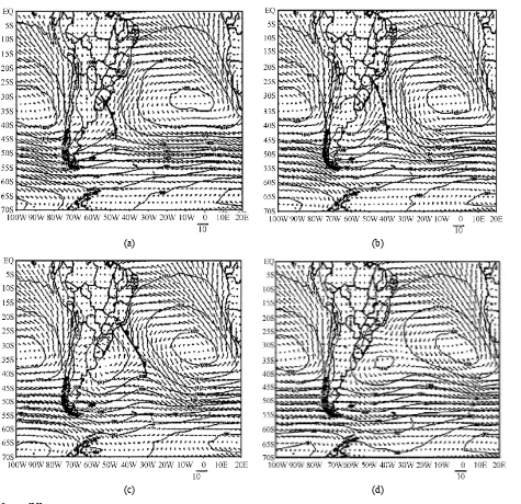
[image:5.595.66.541.81.541.2]Source: [25].
Figure 3. Average fields of sea level pressure (hPa) and 10-m above ground level wind (m/s), for cold fronts passages at (30˚S e 47.5˚W), in summer months. The contour interval is 4 hPa and the location of surface cold front is also marked.
tion processes and their monitoring allows direct esti- mates of the degree of contamination, and obviously making possible their management [27,28].
2.3. Astronomical Tides and Meteorological Residual
The astronomical tide pattern at Arraial do Cabo station is mixed tide. The mixed tides are a type of tide in which the diurnal and semidiurnal oscillations are important factors. The tide is characterized by large differences in height between two high tides (HT) or two consecutive low tides (LT). There are usually two HT and two LT
[image:5.595.304.524.95.424.2]each day, but occasionally the tide can become diurnal.
Figure 5 shows the tidal ranges (vertical distance be- tween high tide and low tide) in Arraial do Cabo that is around 1.20 meter in the largest peaks of low tides due to the diurnal influence, considering periods of spring tide. The semidiurnal constituents M2 (principal lunar) and
S2 (principal solar) have the greatest amplitudes. The
diurnal constituents O1 (principal lunar) and K1 (decli-
national luni-solar) are also present as well as the shallow water constituents M4 (quarter diurnal lunar), MNS2
(se-midiurnal harmonic shallow water) and MS4 (quarter
(a) (b)
(c) (d)
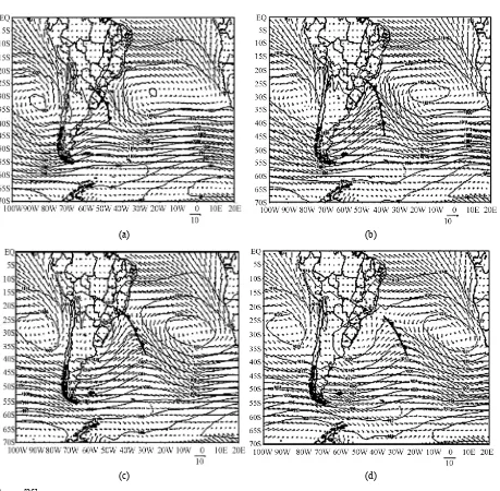
[image:6.595.70.529.74.524.2]Source: [25].
Figure 4. Average fields of sea level pressure (hPa) and 10-m above ground level wind (m/s), for cold fronts passages at (30˚S e 47.5˚W), in the winter months. The contour interval is 4 hPa and the location of surface cold front is also marked.
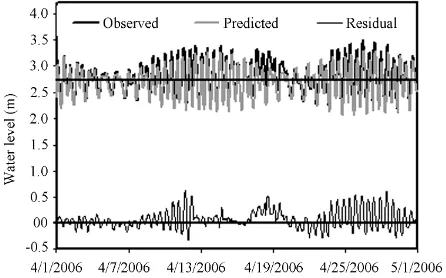
nental shelf [10]. The regular and predictable oscillation of the tides is modified by meteorological patterns, being the principal ones the atmospheric pressure and winds acting on the sea level. These irregular changes, known as surge are the non-tidal residuals and can be defined as the difference between the observed and predicted levels. The non-tidal residual is alternatively called the surge or storm surge, non-tidal component or meteorological re- sidual [10]. Figure 6 shows a 30-day hourly height re- cords of the predicted tide at the Arraial do Cabo tide gauge station, showing the tidal regime with distortions by the influence of the shallow water as well as the observed tide and the variation of the meteorological residual.
Recurrent upwelling events provide cold and rich in
Figure 5. Series of 72 hourly heights of the observed and predicted tides at Arraial do Cabo tide gauge station, start-ing January 1, 2006. It can verify the mixed regime: semi-diurnal with semi-diurnal influence. The smallest peaks of LT characterize this local tidal regime observed on days 1 - 2 at 2300 local time.
Figure 6. Series of harmonic analysis of 720 hourly heights at Arraial do Cabo, observed tide and meteorological resi- dual starting April 1, 2006.
are considered to be driven in large part by predation [31].
2.4. Water Masses in the Southeastern Brazilian Shelf
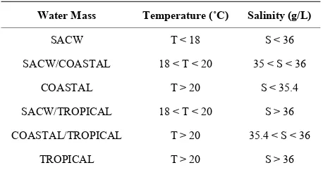
A brief description of the main water masses in the sou-theastern Brazilian shelf is presented in this paper. Tradi-tionally, the classification of water masses is made through temperature/salinity diagrams according to their thermohaline circulation. The water masses can be identi- fied according to the geographic region where they arise, and the depth in which they reach the vertical equilib- rium [6].
The TW is a warm and salty South Atlantic surface water mass, which at the western boundary is transported southward by the BC. This surface water is formed as a result of the intense radiation and excess of evaporation in respect to precipitation. This water mass is character- ized by temperatures above 20˚C and salinities above 36% on Brazilian Southeastern coast [32]. The Sub-Ant- arctic Water is cold and less saline high-latitude water mass and its western boundary layer reaches northward extensions due to advection by the Malvinas Current. These two water masses mix and form the SACW that
takes place at the Subtropical Convergence Zone (con- fluence between the SACW and the Antarctic Circumpo- lar Current) and it extend as far north as 35˚S. The SACW is associated with sinking and northward trans- port and is found flowing into the region of pycnocline, with temperatures above 6˚C and below 20˚C and salini- ties between 34.6 and 36 PSS (Practical Salinity Scale). In the Brazilian Southeast the SACW thermohaline cir- culation is around 20˚C and 36.2 PSS [32]. The Coastal Water (CW) has the thermohaline characteristics varying according to the annual cycle of river runoff and mixture with offshore waters [33]. The Environment National Council (CONAMA) Resolution 357/2005 that provides the classification of water bodies and environmental guidelines for its framework determines limits for the levels of several chemicals components, including ni- trogenous nutrients [16]. We have used temperature and salinity data provided by the Admiral Paulo Moreira In- stitute of Sea Studies—IEAPM and the water mass ther- mohaline indices are presented in Table 1.
2.5. Data
2.5.1. In Situ Measurements
Samples of physical, chemical, and biological surface seawater (0.5 m deep) were collected with a Nansen bot- tle with reverse thermometer outside, and in the bottom (water/sediment interface), by scuba diving using a 2-l polyethylene bottle (three samples). The salinity, dis- solved oxygen, and nutrients were determined ashore as described in [34]. The method described in [35] was ap- plied to chlorophyll a. An inversion thermometer fixed to the outside of a Nansen bottle was employed for tem- perature. Then the physical and chemical parameters are: Sea Surface Temperature (SST), salinity, dissolved oxy- gen (DO), nitrogen as ammonium cation ( ), nitrite (NO2) and nitrate (NO3), and ortho-phosphate (PO4).
+ 4
NH
The biological variables are composed of chlorophyll a
(milligrams per cubic meter) measurements as an esti- mation of microalgal biomass, but probably also contains all free-living autotrophic bacteria of the water column both influenced qualitatively and quantitatively by nutri- ent entrances that on the other hand, supplies itself as feeding material for meroplankton larvae which are ex- pressed in numbers of organisms per cubic meter of wa- ter and were collected by means drag plankton net of 100 mesh and fixed in 10% formalin and then counted under a microscope. These data were collected with weekly frequency from July 21, 1999 to June 28, 2007 in Anjos Bay, Arraial do Cabo city, and the nutrients are in accor- dance with the CONAMA resolution [16].
2.5.2. Meteo-Oceanographic and Sea Level Data Set
1) Station measurements
[image:7.595.61.284.256.395.2]Table 1. Southern Brazilian shelf water mass thermohaline indices in Arraial do Cabo.
Water Mass Temperature (˚C) Salinity (g/L)
SACW T < 18 S < 36
SACW/COASTAL 18 < T < 20 35 < S < 36
COASTAL T > 20 S < 35.4
SACW/TROPICAL 18 < T < 20 S > 36
COASTAL/TROPICAL T > 20 35.4 < S < 36
TROPICAL T > 20 S > 36
tained from the tide gauge station installed at Arraial do Cabo near Anjos Bay at latitude 22˚58'S and longitude 42˚00'W.
The equipment has been operated and maintained by the IEAPM of Brazilian Navy. The tidal predictions were also supplied for the same period. The meteorological residual was obtained from the difference between the observed and predicted levels. 6-hourly (UTC) atmos- pheric pressure and direction and wind speed from São Pedro d’Aldeia (SPA) meteorological station were also used.
2) Satellite wind measurements
The QuikSCAT is the first satellite-borne scanning ra- dar scatterometer which measures the surface roughness of the ocean, affected by the wind magnitude and direc- tion, by transmitting microwave pulses (13.4 GHz) and receiving the backscatter. Multiple and simultaneous normalized radar cross-section values are obtained from the backscatter power at a single geographical location or wind vector cell and converted to wind speed and direc- tion measurements (10 m neutral winds) using a Geo- physical Model Function [36]. High-resolution Quik- SCAT vector wind fields suitable for coastal applications and studying of smaller oceanic processes have been produced by combining scatterometer measurements with a regional mesoscale model [37] or by use of “sli- ces” [38].
The QuikSCAT vector wind product of Remote Sens- ing Systems (RSS) available daily on a 0.25˚ grid was used for the same period, obtained from the National Aeronautics and Space Administration—Jet Propulsion Laboratory—Physical Oceanography Distributed Active Archive Center.
Direction and wind speed as well as the meteorologi- cal residual were calculated from the wind data set and the tide gauge records, respectively. As the surface wind stress provides the most important forcing of the ocean circulation due to the relative motion between the at- mosphere and ocean, we used in this work the zonal (ZWS) and meridional wind stress (MWS) calculated by the following equations:
x d
T C W u (1)
y d
T C W v (2)
where: ρ = 1.22 kg·m−3 (air density);
W = intensity of the wind (m·s−1) calculated from zonal
(u) and meridional (v) wind components; Cd = 1.1 +
0.053W (coefficient of drag for the southeast Brazil coast, [39]). The units used for wind stress are N·m−2, where 1
hPa is equal to 102 N·m−2. The meteo-oceanographic time
series are then weekly and for the same period as all the others.
In this research the physical, chemical and biological parameters were collected with weekly frequency. Astro- nomical tides are one of the most evident sea level oscil- lations, being that the more energetic tides are the semi- diurnal (6-hourly periods) and diurnal (12-hourly periods) and therefore this sample period do not represent the tidal influence when compared with others. Due to the mete- orological systems have longer periods of oscillation and influence the variations in sea level near the coastline, we only used the meteorological residual.
2.6. Methodology 2.6.1. Statistical Analysis
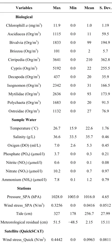
The basic statistical analysis was applied in the environ- mental time series for the period from July 1999 to June 2007. Some outliers were identified and substituted by the average values between the previous and the follow- ing weekly data (Table 2).
Table 2. Statistical summary of the data set.
Variables Max Min Mean S. Dev.
Biological
Chlorophill a (mg/m3) 11.9 0.0 1.0 1.19
Ascidiacea (Org/m3) 1115 0.0 11 59.5
Bivalvia (Org/m3) 1833 0.0 99 194.9
Briozoa (Org/m3) 101 0.0 2 5.7
Cirripedia (Org/m3) 3641 0.0 210 362.8
Cypris (Org/m3) 5192 0.0 22 255.5
Decapoda (Org/m3) 437 0.0 20 35.9
Isognomon (Org/m3) 2342 0.0 31 166.5
Mytilidae (Org/m3) 2636 0.0 93 173.9
Polychaeta (Org/m3) 1683 0.0 20 91.5
Ostreidae (Org/m3) 1132 0.0 27 76.9
Sample Water
Temperature (˚C) 26.7 15.9 22.6 1.76
Salinity (g/L) 36.6 33.5 35.7 0.46
Oxigen (DO) (ml/L) 7.0 2.6 5.3 0.45
Phosphate (PO4) (µmol/l) 3.7 0.0 0.3 0.21
Nitrite (NO2) (µmol/l) 0.6 0.0 0.1 0.08
Nitrate (NO3) (µmol/l) 10.2 0.0 0.7 0.97
Ammonium (NH4) (µmol/l) 7.8 0.1 1.2 0.79
Stations
Pressure_SPA (hPA) 1028.0 1003.0 1016.0 4.65
Wind stress_SPA (N/m2) 0.3256 0.0 0.0416 0.0512
Tide (cm) 327 178 256.7 27.99
Meteorological residual (cm) 51.5 −48.5 2.15 15.11
Satellite (QuickSCAT)
Wind stress_Quick (N/m2) 0.4442 0.0 0.0963 0.0811
2.6.2. Multivariate Statistical Analysis
Cluster analysis is a multivariate technique used to group objects into classes (clusters) on the basis of similarities within a class and dissimilarities between different clas- ses. It is a data classification method. In hierarchical cluster analysis, a dendogram is drawn with samples plotted in clusters on the y axis and linkage distances plotted on the x axis. The linkage distances between the clusters illustrate relative similarities in the characteris- tics of the samples. Ward’s method was used to form the clusters [40]. This method uses an analysis of variance approach to minimize the sum of squares of any two hy-
pothetical clusters. Pearson-r distances were used as the similarity measure. CA is also used to verify the spatial distribution data set and discover groups of similar pat- terns to describe more clearly the structure and composi- tion of the study area ecosystem. The data set was sepa- rated seasonally in spring-summer (upwelling period) and autumn-winter (downwelling period) to characterize which variables are more important in these distinct pe- riods relating them with the sea level variation.
PCA is a technique for mapping multidimensional data into lower dimensions with minimal loss of information. This method can take into account the variability of the data set between different locations (spatial scale) and between successive samples (temporal scale). It is used in all forms of analysis because it is a simple, non-para- metric method of extracting relevant information from data sets. Numerical analysis procedures, such as PCA, have been developed to interpret large space/time data sets, which can decompose total variance into spatial and temporal variances. The principal axis method was used to extract the components, and this was followed by an orthogonal rotation [41]. In environmental studies with many physical, chemical and biological variables, one way to evaluate an integrated complex data is multivari- ate statistical methodology where variables can be ana- lyzed together [42,43]. It consists of a linear transforma- tion of all original variables in new variables or compo- nents. In such a way, the first computed component is responsible for most of the variance in the observed va-riables. The second is responsible for the greatest pos- sible variance remaining and so on until all the variance has been explained. PCA is a variable reduction proce-dure [44]. Then we applied it, which establishes a set of orthogonal factors based on a correlation matrix, provid-ing information about similarities and redundancies of the samples, using Varimax normalized rotation.
3. Results and Discussion in
3.1. Seasonal Variability of the Wind Stress Induced Upwelling
Wind events induce different disturbances in the water mass structure depending on the season. In Arraial do Cabo coastline, when NE-wind events increase the inten- sity for a period, mixing with the water column, the re- sponse is the SACW upwelling with capacity of a redis- tribution of nutrients with effects on plankton dynamics. Considering the seasonality of the wind events that mod-ulates the zonal and meridional wind field, we also veri-fied the number of occurrence of NE and SW wind stress (Figure 7).
that reach the region. Although SPA station presents higher percentage than satellite data set for NE direction, the values are very close between them, around 71% and 62%, respectively. These results show that the Quick Scatterometer winds are also a good source of data set for this coastal area. The predominance of NE winds in- dicates the seasonal variability of the South Atlantic high pressure system that leads upwelling in this region. Therefore the monitoring of this area is important due to the effects that this phenomenon causes in the local bio- diversity and economy.
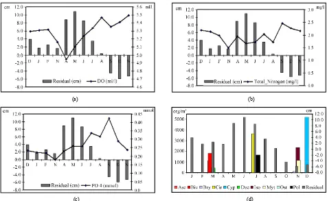
3.2. Seasonal Variability of the Residual and Chemical and Biological Parameters
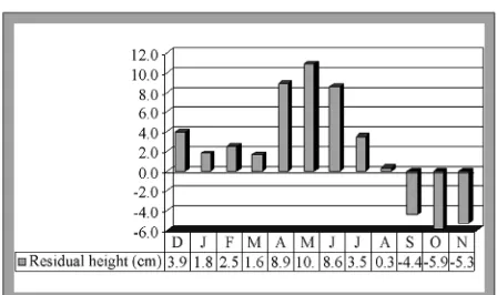
The seasonality of the mean residual presents a well- defined pattern with maximum peaks in the months of autumn and winter. It can be related to the presence of cold fronts that although they reach the region with no much frequency, they are more intense in this period. Another important aspect in raising the sea level is the internal waves due to the interaction of currents, such as barotropic tides and wind-induced flows, including sea- bed topography near the continental shelf [45]. Minimum during spring with negative values and summer can be related to the prevailing of the South Atlantic high-pres- sure with E-N winds blowing offshore the coastline and consequently occurrence of coastal upwelling (Figure 8). Seasonal variations were then compared between mean
[image:10.595.57.289.437.527.2](a) (b)
Figure 7. Number of occurrence of NE (a) and SW (b) wind direction verified at SPA weather station and vector wind obtained by Quick Scatterometer (Q).
Figure 8. Seasonal distribution of the mean values mete- orological residual.
residual, total nitrogen (NO2, NO3, and NH4), DO, PO4,
and peaks of maximum values of larvae. Figure 9 shows an increasing of biological and chemical variables in spring/summer and a minimum of residual which may take place due to the meteorological system previous de- scribed. The opposite is verified in autumn/winter with minimum peaks in April and May. However we can veri- fied that Cirripedia and Polychaeta present maximum in July. In this month verifies the presence of the TW mass which at the western boundary is transported southward by the BC [16]. Cirripedia are sessile invertebrate organ- isms (barnacles) that cover substantial area of the sub- stratum on intertidal and subtidal zones. They live in warm and shallow water and are important in determin- ing and monitoring environmental impacts in coastal areas [46]. Although there are no further reports of eco- nomic damage, it is known that the hulls of ships, oil platforms, pipelines and other plant artificial substrates available in the marine environment may be completely covered by the barnacles causing corrosion of metals and an increase in maintenance costs [47]. The Polychaeta is a bristle-worm with species that live in the coldest ocean temperatures and other which tolerate the extreme high temperatures. An inventory of the species found on the beaches of Rio de Janeiro State, Brazil was made by [48].
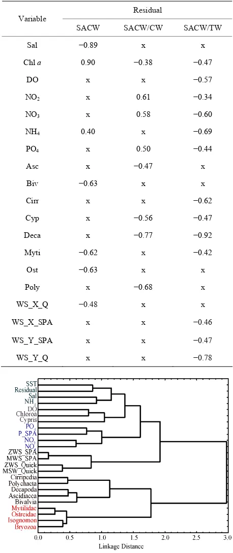
3.3. Cross-Correlations for Different Water Masses
As shown in Table 1, we have used temperature and sa- linity data (thermohaline indices) to classify the water mass. Thus, the data set were separated according to this criterion and applied cross-correlation to verify the rela- tionship between the biological, chemical and physical parameters. Table 3 shows these correlations that were verified only for Central Water (SACW), Central/Coastal Water (SACW/CW) and Central/Tropical Water (SACW/ TW). These correlations verified in the presence of SACW show the importance of this water mass in the coastal upwelling process. In other water masses these variables did not present correlations. Correlation be- tween the residual and the variables in presence of SACW suggest a sensitivity of microorganisms as Bival- via (Class of mussels), Mytilidae (Family of mussels), and Ostreidae (oysters) associated, likely, with the de- crease of the residual due the presence of the South At- lantic Subtropical High (SASH) for the upwelling period with E-NE wind direction. A direct and inverse correla- tion is verified for Chlorophyll a (0.90) and Salinity (−0.89), respectively. The residual also presents direct correlation with the nutrients PO4, NO2 and NO3 for the
[image:10.595.60.284.572.705.2]
(a) (b)
[image:11.595.60.536.84.377.2]
(c) (d)
Figure 9. Seasonal variability of (a) DO, (b) total nitrogen (NO2, NO3, and NH4), (c) PO4, and (d) peaks of maximum values of larvae for 1999-2007 period.
cidiacea, Cypris, Decapoda (−0.77), Polychaeta present a negative correlation with the residual, showing a sensi- bility of these larvae with sea level variations due to me- teorological forcing. For the SACW/TW, the residual presents more correlations with the chemical and bio- logical variables. An inverse correlation with Chlorophyll
a, DO, nutrients, Cirripedia, Cypris and Decapoda (−0.92), suggest also a relation to the same construct. Ascidiacea, Cirripedia and Cypris present correlations for SACW/CW and SACW/TW and are important in studies on recruitment as well as determining and monitoring environmental impacts in coastal regions.
Bivalve mollusks, particularly marine mussels, corre- lated in presence of SACW (−0.63) have been used as indicator organisms in environmental monitoring pro- grammers due to their wide distribution, sedentary life- style, tolerance to a large range of environmental condi- tions and because they are filter-feeders with very low metabolism which allows the bioaccumulation of many chemicals in their tissues [49].
3.4. Multivariate Statistical Analysis
Data grouped according to the CA were performed to verify the structure and composition of the regional eco- system. There are many available algorithms for this task and here we used for the Ward method with Pearson-r
coefficient. Figure 10 illustrates the results of cluster analysis that grouped the sampling points in two big clusters, one of biotic variables in one side and abiotic ones at the other, corresponding to the macrostructure of ecosystem.
The Pearson-r distance was chosen as the similarity measurement, between sampling sites and Ward’s method to form clusters were more successful compared to other methods. Ward’s method is distinct from all other linkage rules because it uses an analysis of variance approach to evaluate the distances between clusters, producing the most distinctive groups [50]. The classification of the samples into clusters is based on a visual observation of the dendrogram at a linkage distance of about line 1.2 (Figure 10). Thus, samples with a linkage distance lower than line 1.2 allows a division of the dendrogram into six clusters, reaching the objectives of the classification me-thod. The degree of refinement of similarities can be written as C1 (family of oysters and mollusks, genus of
marine bivalve mollusks and Bryosoa (phylum of aquatic invertebrate animals as moss animals)), C2 (classes of
barnacles, worms, tunicate, class of mussels and order of crustaceans), C3 (wind), C4 (nitrogen concentration,
phosphorus and pressure), C5 (DO, Chloro a and ostra-
cods (a type of crustacean) C6 (Temperature, Residual,
Table 3. Correlation between the residual and Chemical, Biological and Physical variables (95% confidence interval).
Residual Variable
SACW SACW/CW SACW/TW
Sal −0.89 x x
Chl a 0.90 −0.38 −0.47
DO x x −0.57
NO2 x 0.61 −0.34
NO3 x 0.58 −0.60
NH4 0.40 x −0.69
PO4 x 0.50 −0.44
Asc x −0.47 x
Biv −0.63 x x
Cirr x x −0.62
Cyp x −0.56 −0.47
Deca x −0.77 −0.92
Myti −0.62 x −0.42
Ost −0.63 x x
Poly x −0.68 x
WS_X_Q −0.48 x x
WS_X_SPA x x −0.46
WS_Y_SPA x x −0.47
[image:12.595.59.287.111.651.2]WS_Y_Q x x −0.78
Figure 10. Dendogram for 24-variables illustrating the re- sult of the cluster analysis. Different clusters are indicated by the different colors (C1-C6).
of the zonal and meridional wind variability, including these variables in a single cluster as noted in the first two factors of PCA. In reality, the number of components
extracted in a PCA is equal to the number of observed variables being analyzed. This means that an analysis of N variables would actually result in N components. However, in most analyses, only the first few compo- nents account for meaningful amounts of variance, so only these first few components are retained and inter- preted. In the present study were performed on 24-vari- ables and only eight components were extracted with this criterion. The first component can be expected to have large amount of the total variance. Each succeeding component will account for progressively smaller amounts of variance. Therefore, only the first eight com- ponents were retained and they explain 64.10% of the total variance in the data set. The first three components were the most important, with 15.7%, 11.3% and 8.6% of explained variance (Table 4). The first component was attributed to larvae that had the greatest variability with scores strongly positively correlated to Mytilidae, Deca- poda, Bivalvia, Ostreidae, Isognomon and Bryosoa. This statistical strategy gives greater importance to the larvae in the ordering and feature extraction of the coastal eco- system, being then denominated here “biotic component” that corresponds to the major larvae economically im- portant to the region as crustaceans, mussels and oysters. The second component was strongly negatively corre- lated with zonal and meridional wind from SPA and sat- ellite and relatively weak with meteorological residual (r
= −0.40), showing the interaction sea-air and therefore denominated “wind component”. The third component was attributed to temperature and nutrients. It showed a strong positive correlation with SST and relatively weak positive loading on PO4, NO2 and NO3. These abiotic
Table 4. Correlation between the residual and chemical, biological and physical variables (95% confidence interval).
Factor loading Factor 1 Factor 2 Factor 3 Factor 4
SST 0.105 −0.012 0.716 0.140
Sal 0.020 0.121 0.259 −0.023
DO −0.048 −0.064 −0.306 −0.012
PO4 −0.111 −0.056 −0.532 −0.192
NO2 −0.128 −0.153 −0.560 −0.248
NO3 −0.110 −0.016 −0.535 −0.232
NH4 −0.112 0.096 −0.042 0.014
Chloro a −0.070 −0.115 −0.158 −0.034
Cirripedia 0.383 −0.054 0.115 −0.535
Mytilidae 0.785 −0.251 −0.188 0.257
Decapoda 0.607 −0.220 0.126 −0.368
Polychaeta 0.326 −0.111 0.066 −0.583
Bivalvia 0.668 −0.063 0.117 −0.259
Ostreidae 0.789 −0.251 −0.112 0.187
Cypris 0.079 −0.045 0.033 −0.105
Ascidiacea 0.387 −0.057 0.240 −0.519
Isognomon 0.715 −0.197 −0.132 0.376
Bryozoa 0.595 −0.274 −0.247 0.479
Residual −0.194 −0.400 0.149 0.073
ZWS_SPA −0.310 −0.787 0.090 −0.064
MWS_SPA −0.290 −0.765 0.095 −0.067
P_SPA 0.010 −0.083 −0.439 −0.150
ZWS_Quick −0.278 −0.672 0.150 0.056
MSW_Quick −0.281 −0.718 0.028 0.015
Eigenvalue 3.773 2.711 2.069 1.794
Variability (%) 15.722 11.296 8.619 7.474
Cumulative (%) 15.722 27.019 35.638 43.112
variables, such as C1, C2, C3 and C4 with Factor 1, 2, 3
and 4, corresponding to the importance of the biological variables and local environmental structure.
4. Conclusions
Seasonal variability of the mean meteorological residual presents a well-defined pattern with maximum peaks in autumn and winter and minimum during spring and summer, showing the meaningful meteorological patterns
(a)
(b)
Figure 11. Plot of loadings for the first two components (a), third component (b) with Varimax normalized rotation.
that occur in the region. Comparing the seasonal varia- tions between mean residual, total nitrogen (NO2, NO3,
and NH4), DO, PO4 and larvae we verify that the critical
months with lower values of the residual occur in August, September, October and November. Ascending values of DO are verified from August with maximum peak in November. Total nitrogen and PO4 present high values
from September with maximum peaks. However the lar- vae present peaks in March to Bivalvia, Ascidiacea and Decapoda; July to Cirripedia and Polychaeta when veri- fies the presence of the TW; November to Bryosoa, Isognomon, Mytilidae and Ostreidae and December to Cypris, period of occurrence of upwelling.
[image:13.595.60.283.112.602.2]CA grouped the sampling in two big clusters, one of biotic variables in one side and abiotic ones at the other, corresponding to the macrostructure of ecosystem. The degree of refinement of similarities allowed a division into six clusters of samples, giving the most satisfactory results at forming distinct clusters, reaching thus the ob- jectives of the classification method. This cluster analysis shows the importance not only the biotic variables but also of the zonal and meridional wind variability, includ- ing these variables in a single cluster.
PCA retained and interpreted eight components and they explain 64.10% of the total variance in the data set. The first component was attributed to larvae that had the greatest variability with scores strongly positively corre- lated, corresponding to the major larvae economically important to the region as crustaceans, mussels and oys- ters. The second component was strongly negatively cor-related with zonal and meridional wind both with the SPA station and with satellite wind data and relatively weak with meteorological residual, showing the sea-air coupling. The third component was attributed to tem- perature and nutrients, characterizing the local marine ecosystem related to the presence of different water masses. The fourth factor contributes with a small vari- ance and also relates to the biotic components of the classes of zoobenthos (Cirripedia, Polychaeta and As- cidiacea) found in intertidal zones.
The applied methodology shows the relationship be- tween biological and chemical variables and meteoro- logical processes in the main Brazilian region where up- welling occurs, contributing to the improvement of mod- els of coastal management.
5. Acknowledgements
The authors thank the Admiral Paulo Moreira Institute of Marine Studies—IEAPM of Brazilian Navy for data availability and logistical support. The authors also thank the financial support of the Coordination for the Im- provement of Higher Level Personnel—Brazilian Re- search Agency (Capes).
REFERENCES
[1] P. M. S. Monteiro, G. Nelson, A. van der Plas, E, Mabille, G. W. Baileyd and E. Klingelhoeffer, “Internal Tide-Shelf Topography Interactions as a Forcing Factor Governing the Large-Scale Distribution and Burial Fluxes of Par- ticulate Organic Matter (POM) in the Benguela Upwell- ing System,” Continental Shelf Research, Vol. 25, No. 15, 2005, pp. 1864-1876.
http://dx.doi.org/10.1016/j.csr.2005.06.012
[2] P. M. A. B. Ré, “Biologia Marinha,” Faculdade de Ciên- cias da Universidade de Lisboa, Portugal, 2000.
[3] B. Boehm and S. B. Weisberg, “Tidal Forcing of Entero-
cocci at Marine Recreational Beaches at Fortnightly and Semidiurnal Frequencies,” Environmental Science Tech- nology, Vol. 39, No. 15, 2006, pp. 5575-5583.
[4] F. Pereira, A. L. Belém, M. C. Belmiro and R. Geremias, “Tide-Topography Interaction along the Eastern Brazilian Shelf,” Continental Shelf Research, Vol. 25, No. 12-13, 2005, pp. 1521-1539.
http://dx.doi.org/10.1016/j.csr.2005.04.008
[5] S. A. Piontkovski, M. R. Landry, Z. Z. Finenko, A. V. Kovalev, R. Williams, C. P. Gallienne, A. V. Mishonov, V. A. Skryabin, Y. N. Tokarev and V. N. Nikolsky, “Plankton Communities of the South Atlantic Anticyclo- nic Gyre: Communautés Planctoniques du Tourbillon An- ticyclonique de l’Atlantique Sud,” Oceanologica Acta, Vol. 26, No. 3, 2003, pp. 255-268.
http://dx.doi.org/10.1016/S0399-1784(03)00014-8 [6] R. H. Stewart, “Introduction to Physical Oceanography,”
Texas A & M University, 2007.
[7] D. T. Pugh, “Changing Sea Levels: Effects of Tides, Weather and Climate,”Cambridge University Press, 2005, 265 p.
[8] S. Franco, “Tides: Fundamentals Analysis and Predic- tion,” IPT, São Paulo, 1981.
[9] N. A. Pore, “The Relation of Wind and Pressure to Ex- tratropical Storm Surge at Atlantic City,” Journal of Ap- plied. Meteorology, Vol. 3, No. 2, 1964, pp. 155-163. [10] D. T. Pugh, “Tides, Surges and Mean Sea Level,” John
Wiley & Sons, 1987, 472 p.
[11] D. Prandle and J. Wolf, “The Interaction of Surge and Tide in the North Sea and River Thames,” Geophysical Journal of the Royal Astronomical Society, Vol. 55, No. 1, 1978, pp. 203-216.
[12] J. Wolf, “Surge-Tide Interaction in the North Sea and River Thames, in Floods due to High Winds and Tides,” Elsevier, New York, 1981, pp. 75-94.
[13] K. J. Horsburgh and C.Wilson, “Tide-Surge Interaction and its Role in the Distribution of Surge Residuals in the North Sea,” Journal of Geophysical Research, Vol. 112, No. C8, 2007, pp. 1-13.
http://dx.doi.org/10.1029/2006JC004033
[14] K. Myrberg, O. Andrejev and A. Lehmann, “Dynamic Features of Successive Upwelling Events in the Baltic Sea—A Numerical Case Study,” Oceanologia, Vol. 52, No. 1, 2010, pp. 77-99.
http://dx.doi.org/10.5697/oc.52-1.077
[15] M. M. F. de Oliveira, N. F. Ebecken, de J. L. F. Oliveira and I. A. Santos, “Neural Network Model to Predict a Storm Surge,” Journal of Applied Meteorology and Cli- matology, Vol. 48, No. 1, 2009, pp. 143-155.
http://dx.doi.org/10.1175/2008JAMC1907.1
[16] M. M. F. de Oliveira, G. C. Pereira, J. L. F. de Oliveira and N. F. F. Ebecken, “Large and Mesoscale Meteo- Oceanographic Patterns in Local Responses of Biogeo- chemical Concentrations,” Environmental Monitoring and Assessment, Vol. 184, No. 1, 2012, pp. 6935-6953. http://dx.doi.org/10.1007/s10661-011-2470-3
Ocean,” Oceanography, Vol. 8, No. 3, 1995, pp. 87-91. [18] L. P. Pezzi, “Variabilidade do Sistema Oceano-Atmosfera
no Oceano Atlântico Sudoeste,” I Seminário Sobre Sen- soriamento Remoto Aplicado à Pesca, INPE, S: J: dos Campos, 2006.
[19] M. A. Guimaraens and R. Coutinho, “Spatial and Tem- poral Variation of Benthic Marine Algae at the Cabo Frio Upwelling Region,” Aquatic Botany,Vol.52, No. 4, 1996, pp. 283-299.
http://dx.doi.org/10.1016/0304-3770(95)00511-0
[20] G. C. Pereira, R. Coutinho and N. F. F. Ebecken, “Data Mining for Environmental Analysis and Diagnostic: A Case Study of Upwelling Ecosystem of Arraial do Cabo,” Brazilian Journal of Oceanography,Vol. 56, No. 1, 2008, pp. 1-18.
[21] C. D. Ahrens, “Meteorology Today: An Introduction to Weather Climate and the Environment,” 6th Edition, Brooks/Cole, London, 2000.
[22] R. B. de. Souza, “Oceanografia por Satélites,” 2nd Edi- tion, Oficina de Textos, São Paulo, 2008.
[23] S. A.Gaeta, J. A. Lorenzetti, L. B. Miranda, S. M. M. Susimi-Ribeiro, M. Pompeu and C. E. S. Araújo, “The Vitória Eddy and Its Relation to the Phytoplankton Bio- mass and Primary Production during the Austral Fall of 1995,” Archive of Fishery and Marine Research, Vol. 47, No. 2-3, 1999, pp. 253-270.
[24] R. P. Matano, M. Schlax and D. B. Chelton, “Seasonal Variability in the Southwestern Atlantic,” Journal of Geophysical Research, Vol. 98, No. C10, 1993, pp. 18027- 18035.
[25] M. L. G. Rodrigues, D. Franco and S. Sugahara, “Clima- tologia de Frentes Frias no Litoral de Santa Catarina,” Revista Brasileira de Geofísica,Vol. 22, No. 2, 2004, pp. 135-151.
http://dx.doi.org/10.1590/S0102-261X2004000200004 [26] J. L. Valentin, “The Dynamics of Plankton in the Cabo
Frio Upwelling,” In: F. P. Brandini, Ed., Memórias do III EBP, Caiobá-Curitiba, 1989.
[27] D. Topcu, H. Behrendt, U. Brockmann and U. Claussen, “Natural Background Concentrations of Nutrients in the German Bight Area (North Sea),” Environment Monitor- ing and Assessment, Vol. 174, No. 1-4, 2010, pp. 361-388. http://dx.doi.org/10.1007/s10661-010-1463-y
[28] R. P. Morgan and K. M. Kline, “Nutrient Concentrations in Maryland Non-Tidal Streams,” Environment Monitor- ing and Assessment, Vol. 178, No. 1-4, 2011, pp. 221-235. http://dx.doi.org/10.1007/s10661-010-1684-0
[29] M. Ribas-Ribas, J. M. Hernández-Ayón, V. F. Cama- cho-Ibar, A. Cabello-Pasini, A. Mejia-Trejo, R. Durazo, S. Galindo-Bect, A. J. Souza, J. M. Forja and A. Siqueiros- Valencia, “Effects of Upwelling, Tides and Biological Processes on the Inorganic Carbon System of a Coastal Lagoon in Baja California,” Estuarine, Coastal and Shelf Science, Vol. 95, No. 4, 2011, pp. 367-376.
http://dx.doi.org/10.1016/j.ecss.2011.09.017
[30] R: N. Gibson, “Go with the Flow: Tidal Migration in Marine Animals,” Hydrobiologia, Vol. 503, No. 1-3, 2003, pp. 153-161.
http://dx.doi.org/10.1023/B:HYDR.0000008488.33614.6 2
[31] J. K. Breckenridge and S. M. Bollens, “Vertical Distribu- tion and Migration of Decapod Larvaein Relation to Light and Tides in Willapa Bay,” Estuaries and Coasts, Vol. 34, No. 6, 2011, pp. 1255-1261.
http://dx.doi.org/10.1007/s12237-011-9405-7
[32] C. A. Silveira, A. C. K. Schimidt, E. J. D. Campos, S. S. Godoi and Y. Ikeda, “The Brazil Current off the Eastern Brazilian Coast,” Brazilian Journal of Oceanography, Vol. 48, No. 2, 2000, pp. 171-183.
http://dx.doi.org/10.1590/S1413-77392000000200008 [33] I. Soares and O. M.oller Jr., “Low-Frequency Currents
and Water Mass Spatial Distribution on the Southern Bra- zilian Shelf,” Continental Shelf Research, Vol. 21, 2001, pp. 1785-1814.
[34] SCOR, “Protocols for the Joint Global Ocean Flux Study (JGOFS) Core Measurements,” Scientific Committee on Ocean Research, International Council of Scientific Un-ions, Bergen, Vol. 9, 1996, 170 p.
[35] T. A. Richard and T. G. Thompson, “The Estimation and Characterization of Plankton Population by Pigment Ana- lyses. A Spectrophotometric Method for the Estimation of Plankton Pigments,” Journal of Marine Research, Vol. 11, 1952, pp. 156-172.
[36] N. Sharma and E. D’Sa, “Assessment and Analysis of QuikSCAT Vector Wind Products for the Gulf of Mexico. A Long-Term and Hurricane Analysis,” Sensors, Vol. 8, No. 3, 2008, pp. 1927-1949.
http://dx.doi.org/10.3390/s8031927
[37] Y. Chao, Z. Li, J. C. Kindle, J. D. Paduan and F. P. Chavez, “A High-Resolution Surface Vector Wind Prod- uct for Coastal Oceans: Blending Satellite Scatterometer Measurements with Regional Mesoscale Atmospheric Model Simulations,” Geophysical Research Letters, Vol. 30, No. 1, 2003, pp. 1-13.
http://dx.doi.org/10.1029/2002GL015729
[38] W. Tang, W. T. Liu and B. W. Stiles, “Evaluation of High-Resolution Ocean Surface Vector Winds Measured by QuikSCAT Scatterometer in Coastal Regions,” IEEE Transactions on Geoscience and Remote Sensing, Vol. 42, No. 8, 2004, pp. 1762-1769.
http://dx.doi.org/10.1109/TGRS.2004.831685
[39] J. L Stech and J. A. Lorenzzetti, “The Response of the South Brazil Bight to the Passage of Wintertime Cold Fronts,” Journal of Geophysics Research, Vol. 97, No. C6, 1992, pp. 9507-9520.
[40] S. Sharma, “Applied Multivariate Techniques,” John Wiley and Sons, Inc., New York, 1996.
[41] H. Abdi and L. J. Williams, “Principal Component Anal- ysis,” Wiley Interdisciplinary Reviews: Computational Statistics, Vol. 2, No. 4, 2010, pp. 387-515.
http://dx.doi.org/10.1002/wics.101
http://dx.doi.org/10.1016/j.marpolbul.2010.10.006 [43] M. Ujević Bošnjak, K. Capak, A. Jazbec, C. Casiot, L.
Sipos, V. Poljak and Ž. Dadić, “Hydrochemical Charac-terization of Arsenic Contaminated Alluvial Aquifers in Eastern Croatia Using Multivariate Statistical Techniques and Arsenic Risk Assessment,” Science of the Total En- vironment, Vol. 420, 2012, pp. 100-110.
http://dx.doi.org/10.1016/j.scitotenv.2012.01.021
[44] J. V. E. Bernardi, L. D. Lacerda, J. G. Dórea, P. M. B. Landim, J. P. O. Gomes, R. Almeida, A. G. Manzatto and W. R. Bastos, “Aplicação da Análise das Componentes Principais na Ordenação dos Parâmetros Físico-Quimicos no Alto Rio Madeira e Afluentes, Amazônia Ocidenta,” Geochimica Brasiliensis, Vol. 23, No. 1, 2009, pp. 79-90. [45] A. Stigebrandt, “Resistance to Barotropic Tidal Flow in
Straits by Baroclinic Wave Drag,” Journal of Physical Oceanography, Vol. 29, No. 2, 1999, pp. 191-197. [46] M. Apolinário, “Variation of Populations Densities be-
tween Two Species of Barnacles (Cirripedia: Megab- ala-ninae) at Guanabara Bay and Nearly Islands in Rio de Janeiro/RJ,” Nauplius, Vol. 9, No. 2, 2001, pp. 21-30. [47] M A. Champ and F. L. Lowenstein, “TBT—The Dilem-
ma of High-Technology Antifouling Paints,” Oceanus, Vol. 35, 1987, pp. 69-77.
[48] M. B. Rocha, V. Radashevsky and P. C. Paiva, “Espécies de Scolelepis (Polychaeta, Spionidae) de Praias do Estado do Rio de Janeiro, Brasil,” Biota Neotrópica, Vol. 9, No. 4, 2009.
http://dx.doi.org/10.1590/S1676-06032009000400012 [49] S. M. Lima, J. R. Moreira, A. V. Von Osten, M. Soares
and L. Guilhermino, “Biochemical Responses of the Ma- rine Mussel Mytilus galloprovincialis to Petrochemical Environmental Contamination along the North-Western Coast of Portugal,” Chemosphere, Vol. 66, No. 7, 2007, pp. 1230-1242.
http://dx.doi.org/10.1016/j.chemosphere.2006.07.057 [50] StatSoft Inc., “Statistica,” Data Analysis Software System,
version 7, 2004.
[51] B. Torrano-Siva, “Fitobentos (Macoalgas) in: Informe Sobre as Espécies Exóticas Invasoras Marinhas no Bra- sil,” Ministério do Meio Ambiente, MMA, 2009. [52] S. A. Narandio, J. L. Carvalho and J. C. García-Gomes,
“Effects of Environmental Stress on Ascidians Popula- tions in Algeciras bay (Southerm Spain),” Marine Ecol- ogy, Vol. 144, 1996, pp. 119-131.
[53] T. C. C. Lambert and G. Lambert, “Non-Indigenous As- cidians In southerm California Harbors and Marinas,” Marine Biology, Vol. 130, No. 4, 1998, pp. 675-688. http://dx.doi.org/10.1007/s002270050289