Munich Personal RePEc Archive
Exploiting price misalignements
Rambaccussing, Dooruj
University of Exeter Business School
9 September 2009
Online at
https://mpra.ub.uni-muenchen.de/27147/
Exploiting Price Misalignments
Dooruj Rambaccussing
yUniversity of Exeter
09 Sep 2009
Abstract
This paper de…nes and tests a simple passive trading strategy which involves comparing the price of an asset with its fundamental value. The fundamental value is computed from the real-time forecasts of dividends, expected returns and dividend growth rate using simple regression schemes. By de…ning a measure of going long in either the equity or the bond mar-ket, the rule is found to signi…cantly outperform the passive Buy and Hold strategy with stronger e¤ect in longer horizons. The returns from the strategy also tend to vary with the forecasting model and the de…ni-tion of the discount rate in the present value relade…ni-tion.
Key Words: Dividend Forecasting, Trading Rule, Net Present Value JEL References: G12, G14, G17
1
Introduction
A classic proposition of equilibrium search in asset pricing requires that agents attempt to exploit arbitrage opportunities if they exist and happen to be known. In such a case, the market prices will not re‡ect the net value of the asset. Misalignments between the actual price and the corresponding net present value may o¤er pro…t opportunities, which may be arbitraged away as the actual prices revert to the net present value. For instance, if prices are higher than the net present value, it would mean that the asset is overpriced and over time, there should be a downward reversion towards the fundamentals On the other hand, if prices are lower than the net present value, under the aggregated expectations of agents in the market, there should be an upward dynamic adjustment. A simple trading rule in such a circumstance would be to hold the asset when it is underpriced and sell it if it is overpriced.
While the actual price is observable, the empirical problem lies in computing the fundamental value. According to standard asset pricing theory, the price of any asset is the discounted conditional expectations of future payo¤s. In the case of the stock price, usually the fundamental price is translated into the net present value of the expected future streams of dividends and the terminal equity price. However at a particular time t, the expected future dividends is unknown. Similar to the learning literature, the data generating process for dividends being unknown, agents are assumed to use econometric models to forecast dividends. Empirically, three simple linear econometric models that an agent may reckon to be the data generating process, are used to forecast one step ahead in each period, and the forecast is used to proxy the expected future dividends. Hence model uncertainty is not tackled in this work. For an inter-esting overview of model uncertainty in the context of net present value, see
Avramov (2002,2004), Timmermann and Granger (2004),
Timmer-mann (1993,1996), Pesaran and TimmerTimmer-mann(1995,2002), Rey(2005) The stochastic discount rate and dividend growth rate are computed using the same approach. The forecast variables are then used to arrive to the rational expectations net present value.
The trading rule is built up based on the above principle, which assumes real-time. The real- time construct of the fundamental price (net present value) implies that the net present value is built up at time t, with data available only at that point of time. Empirically, adapted information set of agents is translated through the use of the of expanding and rolling windows. A further advantage, besides the theoretical nature of informations sets is that rolling and expanding windows tend to reduce parameter uncertainty and estimation risk in large samples. Another model to take into account the real-time nature of series
includeRambaccussing (2010) andKoijen and Van Binsbergen(2010).
been documented (Shiller and Beltratti (1993), Poterba and Summers (1988)).
2
Related Literature
The trading rule is built in line with equilibrium search theory in asset pric-ing. The main gist of the rule is to identify periods when the equity market is mispriced and sequentially decide whether to hold equity or bonds conditional on the direction of the mispricing. The simple idea is that if the actual price at time t is higher than the net present value, wealth is held in bonds. The argument for doing so is simply because of the potential capital losses that will be made when actual prices revert back to their fundamental values. On the other hand, if prices are lower than the fundamental price, when asset prices are rise to the fundamental value, capital gains can be made. The rule is a market timing mechanism that enables the agent to shift his wealth from bond to equity assets and vice versa.
Bulkley and Tonks (1989) used a similar version of the rule as a test
of weak form e¢ciency for the UK market. They also showed that revision in the parameters of an econometric model of dividends may explain excess volatility in prices. Improper estimates of the parameters of the dividend model were found to be strong enough to generate strong e¤ects on the stock index price. The rule was tested was tested against the Buy and Hold Strategy for the
S&P 500 market with the same outcome as in the UK market (Bulkley and
Tonks (1992)) The rule was also found to have a lower risk than the simple
Buy and Hold Strategy. Taylor and Bulkley (1996) use the same REPV
formulae in a Price conditional VAR model to derive the theoretical price. The objective however was to test whether underpriced portfolios tend to generate higher returns than overpriced portfolios over several years horizon going until 10 years.
Unlike earlier studies, our major contribution lies in applying real time con-cept to the rule. We allow for 3 models as being the data generating process of dividends which an agent may usually apply, and allow for the update of the parameters based on the information set through the use of moving estimation windows. Our rule assumes that agents may actually forecast based on their information set. We also impose empirical time variation on the discount rate by computing the expected returns as a simple rolling and recursive mean. We also use two de…nitions of the discount rate based on cointegration between
3
Model
From basic asset pricing theory, the price of an asset is equal to the Euler equation or …rst order conditions from a utility optimizing agent faced with a set of intertemporal choice problems. The simple empirical construct of the net present value model or fundamental price for the equity index can be written as:
Pt =
1
Et[rt+1 gt+1]
Et[Dt+1] (1)
where rt+1 is the stochastic discount rate at time t+ 1 and gt+1 is the
dividend growth rate. Et[Dt+1]is the expected future dividend at timet. The
rule posits comparing 1 with the actual price at time t, to determine whether to go long on bonds:
Pt > Pt :Go Long on Bond Market
Pt < Pt :Go long on Equity Market
The empirical cornerstone of the model is to estimate the components of equation 1. The variables are estimated according to di¤erent econometric mod-els based on both rolling and recursive windows. Moving windows, as mentioned previously allow for two interesting advantages. Firstly, it is in line with real time market timing decisions. Agents make their decision to shift their wealth
based on the information they have at timet. The other advantage of allowing
parameters to be updated sequentially is that estimates are more robust in the presence of structural and parameter instability. Recursive windows, allow the information set to grow with each new observation of the variable of interest in the market. It is more suited to cases when the parameters of the regression model do not vary a lot through time. Rolling windows on the other hand, take into account a …xed block of observations (the information set), for estimat-ing the models. If window length of the rollestimat-ing estimate is large and there are no strong variability in parameter estimates, the di¤erence in forecast between rolling and recursive windows might be marginal.
3.1
Models for forecasting Dividends
seasonal dummies, may have its imperfections; however, the bene…ts of apply-ing the rule to a monthly frequency exceeds the e¤ects of marginal seasonality estimation problems.
The three models that are used to forecast dividends are provided as follows:
Dt+1= 0(t+1)+ 12
X
i=1
iIi+ p
X
i=0
iDt i+ 1 D
P t 1+ 2 E
P t 1+ 3(E E )t 1+"t+1
(Model 1a)
lnDt+1 = 0(t+1)+ 12
X
i=1
iIi+ p
X
i=0
ilnDt i+ 1ln D
P t 1+ 2ln E
P t 1+ 3ln(E E )t 1+"t+1
(Model 1b)
Model 1 is an ARMAX model where the exogenous inputs are the macro-economic series Dividend - Price Ratio, Earnings- Price Ratio and a measure of Okun’s gap which is taken to be the deviation of actual earnings from the trended mean earnings. The model also contains a trend and the seasonal dum-mies. The optimal number of lags p is chosen by the Akaike criteria on the di¤erenced form of the equation (due to the presence of unit roots).
Dt+1= 0(t+ 1) + 12
X
i=1
iIi+ p
X
i=0
iDt i+"t+1 (Model 2a)
lnDt+1= 0(t+ 1) + 12
X
i=1
iIi+ p
X
i=0
ilnDt i+"t+1 (Model 2b)
Models 2 are a nested form of Model 1, with the corresponding gamma parameters ( )set to zero.
Dt+1= 0(t+ 1) + 12
X
i=1
iIi+"t+1 (Model 3a)
lnDt+1= 0(t+ 1) + 12
X
i=1
ilnIi+"t+1 (Model 3b)
3.2
Stochastic Discount Factor and Dividend Growth Rates.
In this section, we describe four simple models to construct of the denominators for equation 1. The denominators are very important since minor changes may lead to extremely large changes in the fundamental price, in‡uencing the deci-sion of whether to go long on bonds or equity. The …rst two measures simply use recursive and rolling estimation of the mean of past realized returns. The next two models may be applied in the presence of cointegration between dividends and price.
The Rolling Discount rate is the moving average of realized returns over time for a period of 30 years. For instance the average returns over time at a particular datet will be average returns over the past 30 years. This is given by:
E(rt+1) = 1
360 t
X
i=t 360
Rt (2)
whereRi is the realized returns on the market and t is the terminal date.
The recursive discount rate is the average of realized returns from the be-ginning of the sample(January 1871)until time t.
E(rt+1) = 1 N
t
X
i=t N
Ri (3)
whereN 360:
Denominators A and B include the Recursive Dividend Growth Rate (g) which is de…ned as follows
E(gt+1) =
1
N
t
X
T=t N
ln( DT
DT 1
) (4)
Hence the denominators A and B can be rewritten as such :
rt gt= 1 360
t
X
T=t 360 RT
1
N
t
X
t=t N
ln( DT
DT 1) (A)
rt gt= 1
N
t
X
T=t N
RT 1
N
t
X
T=t N
ln( DT
DT 1
) (B)
Fama and French (2002)show that if the dividend price ratio is
dividend price ratio has ‡uctuating periods of stationarity Appendix A.9 o¤ers a small discussion of the stationarity of the two di¤erent variables.
rt= 1
N
t
X
T=t N
DT
PT 1
+ 1
N
t
X
T=i N
ln( DT
DT 1
) (5)
As in the case of the Dividend growth rate, the Earnings growth rate can be used with the dividend price ratio to derive the discount rate.
rt= 1
N
t
X
T=t N
DT
PT 1
+ 1
N
t
X
t=T N ln( ET
ET 1
) (6)
The next denominators include the Fama and French de…nitions of the dis-count rates with the recursive growth rate as de…ned in4. Model G is the Fama and French discount rate using dividend growth rate while model H is the Fama and French Model using the Earnings growth rate. Model G can be seen to
revert back to the discount factor de…nition adopted byBulkley and Tonks
(1989)but in a time varying context.
rt gt= 1
N
t
X
t=T N
DT
PT 1
+ 1
N
t
X
t=T N ln( ET
ET 1
) 1
N
t
X
t=T N ln( ET
ET 1
)
Using the dividend yield framework, the denominator proxies average real-ized returns and can be seen to revert to :
rt gt= 1
N
t
X
t=T N
DT
PT 1
(C)
The denominator using the Earnings yield is given by D, which is more of a measure of expected returns
rt gt= 1
N
t
X
t=T N
DT
PT 1
+ 1
N
t
X
t=T N ln( ET
ET 1
) 1
N
t
X
t=T N
ln( DT
DT 1
) (D)
4
Data and Results
4.1
Data
used is from Robert Shiller. Forecasts were generated from January 1901 on-wards on a rolling and a recursive basis to December 2007. The risk free rate of return was proxied by the long interest rate again provided by Shiller. We use data from 1871:01 to 1900:12 as the initial estimation sample, and retain the period from 1901:01 to 2007:12 as the out of sample evaluation period. The …rst window approach is the recursive which uses the estimation sample of 1871:01 until one month prior to the one step ahead forecast. For instance the one step ahead forecast of 1940:01 uses the estimation sample of 1901:01 until 1939:12. The second rolling window approach uses a …xed length window of the most recent 30 years of monthly data to estimate the parameters of the model and then forecasts dividends conditional on these parameter estimates. As such the signi…cance of the insample parameter estimates are not tested for economic signi…cance.
4.2
Results
We report the cumulated returns from the initial date of forecast to the terminal date (1900-2008) and average returns over 12, 24, 36, 48 and 60 months. The average return under the Buy and Hold and Trading strategy is as follows :
RBH(k) = 1
T k
T k
X
h=1
K
Y
i=h k
(1 +Rm;i) (7)
RT R(k) = 1
T k
T k
X
h=1
K
Y
i=h k
(1 +Rtr;i) (8)
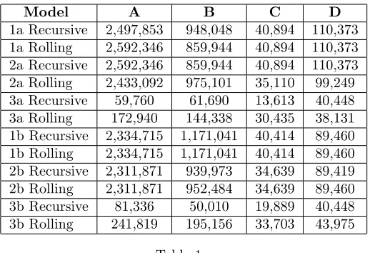
Model A B C D
1a Recursive 2,497,853 948,048 40,894 110,373
1a Rolling 2,592,346 859,944 40,894 110,373
2a Recursive 2,592,346 859,944 40,894 110,373
2a Rolling 2,433,092 975,101 35,110 99,249
3a Recursive 59,760 61,690 13,613 40,448
3a Rolling 172,940 144,338 30,435 38,131
1b Recursive 2,334,715 1,171,041 40,414 89,460
1b Rolling 2,334,715 1,171,041 40,414 89,460
2b Recursive 2,311,871 939,973 34,639 89,419
2b Rolling 2,311,871 952,484 34,639 89,460
3b Recursive 81,336 50,010 19,889 40,448
[image:10.612.177.436.122.299.2]3b Rolling 241,819 195,156 33,703 43,975
Table 1:
Table 1 displays the return on £100 in December 2007 if it were invested back in January 1900 for the di¤erent forecasting models and denominators.
Based on the terminal wealth, each forecasting model have mixed success with regards to the adoption of wealth. The highest wealth is reached through denominator A and model 1a Rolling and 2a Recursive. On average forecasting models 1 and 2 tend to perform very well, irrespective of the functional form. We also report the total compounded monthly returns for periods of 12, 24, 36, 48 and 60 months in appendix A. The success of the rule tends to vary under the di¤erent forecasting models, de…nitions of discount rates and to a lesser extent, the time horizon the rule put to use. The trading rule, when put to use, under the 12, 24, 36, 48 and 60 months horizons beat the naive buy and hold strategy 50 % , 48% , 58.3 % , 56.25 % and 56.25 % of the time. There is no easily tractable di¤erence between the recursive and rolling window performance. All across the di¤erent discount rates, it is found that the best ranking de…nition of the discount rates are A, B, D and C. There appears to be some uniformity over time on the better performing forecasting model and discount rates. For longer periods of adopting the rule, the di¤erence in the cumulated returns tend to increase within the forecasting models and the denominators.
wealth level would be achieved by shifting to the bond market. Appendix 2 shows the graphical plot of wealth for the di¤erent models and denominators over time.
Historically, model 3 postulates a long position in the equity market until 1914. Afterwards, the rule suggests going long on bond markets until 1927and also during 1932- 1936. Interestingly, it takes advantage of the growth of the equity market during the period 1949-1974. The shocks of 73/74 are predicted after the shock and this leads to the rule postulating going long on the bond market. Models 1 and 2 tend to switch more often and the switches appear to be independent over time. This may be explained by the forecasting success of the models where by the forecasting error tends to be more normally distributed with the mean zero. In a random year, switching may occur 3-5 times, as opposed to only once in the model 1. The rule postulates that going long on bond from 1917 to 1927. The rule posits going long on equity from 1927-1931, and in bonds from 1932 till 1936, taking a late advantage of the great depression. Again the rule exploits the growth of the equity markets during the 50’s and 60’s. However, it is a late predictor of the 73/74 shocks where the rule postulates going long on the equity market. However, it later involves investing in the bond market during 75-76. and 80-84. Afterwards, it postulates going long on the equity market.
Generally, the de…nition of the discount rate based on the fundamentals tends to advise ‘going long’ more often. An interesting phenomenon that is encountered, especially when using the Fama and French discount rates, models 1 and 2 do not switch as often in a particular year. They tend to exhibit periods of dependence. The discount rate based on the fundamentals is so small that it o¤sets the serially uncorrelated forecast error. In other words, although the forecast from models 1 and 2 are more accurate (and hence more proned to under or over forecast realized dividends), the discount rate is su¢ciently low such that the accuracy of the forecast vis a vis the true data generating process, does not matter. It is worth noting that there is an improvement in the accuracy of the forecast models at that time. Better forecasting leads to higher wealth, at least for denominators A and B.
4.2.1 Reliability of the Rule
the rule starts dominating the Buy and Hold strategy. Two types of risks are involved in the trading strategy. Over the holding period, riskiness may emanate from the variations in both the equity and bond market. In appendix 4,we report the Sweeney statistic which is designed to account for the time an asset is held in stocks and in bonds. The Sweeney statistic demonstrates that the strategy works better conditional on the denominator adopted.
When transaction costs were accounted for, the number of models beating the market returns fall drastically. In the worst case scenario, when a monthly transaction cost of 0.5 % is implicitly assumed, only eight models beat the market return, mostly from denominators A and B. The Fama and French de-nominators do not yield a favorable outcome in any of the transaction cost. The results are derived by netting the trading rule returns with the transaction costs and computing the Sweeney Z statistic (Appendix 4).
Potential data mining problems are dealt in this study by performing a Monte Carlo simulation of di¤erent times when the rule is put to use. The Monte Carlo simulation involves picking out random dates from the period 1900 to an end date which is conditional on the performance horizon we want to investi-gate. The selection of the random dates is derived from a uniform probability distribution. A vector of dates is generated using a random number generator where an equally size vector between zero and one is randomly chosen from the uniform probability distribution. This vector is then multiplied with n-k where n is the end date of the sample and k is the length of horizon we are looking at, for example k = 12, 24. . . ..60. Subtraction of k ensures that returns under the passive Buy and Hold can be calculated for horizon k, especially if the draw is near the end of the sample. The results (Appenix 8) from the Monte Carlo simulation are not di¤erent from those of the Trading Rule. Models 1 and 2 are the best performers, when coupled with denominators A and B. In the one year horizon, the rule beats the passive buy and Hold only 41 % of the times. However it is worth noting that in the one year period, there are many instances when the rule is equal to the Buy and Hold market return. As the holding pe-riod is increased, the number of times the rule beats the market return tends to increase as well. The rule is better for years 3,4 and 5.
5
Conclusion
empirical de…nitions of the discount rate seem to be better …tted in computing the theoretical price. Both transaction costs and risk tend to reduce the costs.
The strategy put forward also ensures that there are lower risks.than the Buy and Hold Strategy since wealth is at times kept in the bond market which exhibits lower volatility. The only problem with the model which tends to switch the asset more often yields higher transaction costs. The present study may be amended and re…ned in various ways. Various linear and non linear models may be used to forecast dividends in the present framework. A more robust analysis might be conducted to see whether more switches, from the di¤erent models might lead to higher wealth.
References
[1] Doron Avramov,Stock return predictability and model uncertainty, Journal
of Financial Economics64(2002), no. 3, 423 – 458.
[2] Doron Avramov,Stock return predictability and asset pricing models, The
Review of Financial Studies17(2004), no. 3, 699–738.
[3] George Bulkley and Nick Taylor, A cross-section test of the present value
model, Journal of Empirical Finance2(1996), no. 4, 295 – 306.
[4] George Bulkley and Ian Tonks, Are uk stock prices excessively volatile?
trading rules and variance bound tests, The Economic Journal 99 (1989), no. 398, 1083–1098.
[5] George Bulkley and Ian Tonks, Trading rules and excess volatility, The
Journal of Financial and Quantitative Analysis27 (1992), no. 3, 365–382.
[6] Francis X. Diebold and Roberto S. Mariano, Comparing predictive
accu-racy, Journal of Business and Economic Statistics13 (1995), no. 3, 253–
263.
[7] Eugene F. Fama and Kenneth R. French,The equity premium, The Journal
of Finance 57(2002), no. 2, 637–659.
[8] Hashem Pesaran, Davide Pettenuzzo, and Allan Timmermann, Learning,
structural instability, and present value calculations., Econometric Reviews 26 (2007), no. 2-4, 253 – 288.
[9] James M. Poterba and Lawrence H. Summers, Mean reversion in stock
prices : Evidence and implications, Journal of Financial Economics 22 (1988), no. 1, 27 – 59.
[10] David Rey,Market timing and model uncertainty: An exploratory study for
[11] Robert J. Shiller and Andrea E. Beltratti, Stock prices and bond yields: Can their comovements be explained in terms of present value models?, (1993).
[12] Richard J. Sweeney,Beating the foreign exchange market, The Journal of
Finance 41(1986), no. 1, 163–182.
[13] A. Timmermann, Elusive return predictability, International Journal of
Forecasting 24(2008), no. 1, 1–18.
[14] Allan Timmermann and Clive W. J. Granger,E¢cient market hypothesis
and forecasting, International Journal of Forecasting20(2004), no. 1, 15 – 27.
[15] Allan G. Timmermann, How learning in …nancial markets generates
ex-cess volatility and predictability in stock prices, The Quarterly Journal of
Economics 108(1993), no. 4, 1135–1145.
[16] Jules H. Van Binsbergen and Ralph S. Koijen,Predictive Regressions: A
A
Appendix
A.1
Cumulated Monthly Returns
12 Months 24 Months 36 Months 48 Months 60 Months
Model A B C D A B C D A B C D A B C D A B C D
[image:15.612.104.777.189.372.2]1a Recursive 11.2 10.1 6.9 8.5 23.6 21 14.4 17.7 37.5 33.2 22.2 27.5 53.6 46.9 30.7 38.5 71 61.4 39.6 50 1a Rolling 11.2 10 6.9 8.5 23.7 20.8 14.4 17.7 37.7 32.9 22.2 27.5 53.8 46.5 30.7 38.5 71.3 60.9 39.6 50 2a Recursive 11.2 10 6.9 8.5 23.7 20.8 14.4 17.7 37.7 32.9 22.2 27.5 53.8 46.5 30.7 38.5 71.3 60.9 39.6 50 2a Rolling 11.1 10.1 6.7 8.4 23.5 21.1 14.1 17.5 37.4 33.4 21.7 27.1 53.2 47.2 29.9 38.0 70.4 61.9 38.6 49.3 3a Recursive 7.4 7.4 5.8 7.4 15.5 15.4 12.1 15.5 24.2 23.9 18.6 24 33.6 33.0 25.5 33.3 43.9 43 32.6 42.9 3a Rolling 8.3 8.3 6.6 7.4 17.4 17.1 14.0 15.5 27.4 26.8 21.7 24.2 38.1 37.2 29.9 33.5 49.7 48.3 38.6 43.1 1b Recursive 11.1 10.3 6.9 8.3 23.4 21.6 14.4 17.2 37.2 34.3 22.2 26.8 52.9 48.4 30.6 37.5 70.2 63.6 39.5 48.6 1b Rolling 11.1 10.3 6.9 8.3 23.4 21.6 14.4 17.2 37.2 34.3 22.2 26.8 52.9 48.4 30.6 37.5 70.2 63.6 39.5 48.6 2b Recursive 11.1 10 6.7 8.3 23.4 21.1 14.1 17.2 37.3 33.4 21.7 26.8 53.2 47.1 29.9 37.5 70.5 61.9 38.5 48.6 2b Rolling 11.1 10.1 6.7 8.3 23.4 21.1 14.1 17.2 37.3 33.4 21.7 26.8 53.2 47.2 29.9 37.5 70.5 62 38.5 48.6 3b Recursive 11.1 10.3 6.9 8.3 15.8 14.9 12.8 15.5 24.6 23.1 19.8 24.0 34 31.9 27.1 33.3 44.3 41.6 34.8 42.9 3b Rolling 11.1 10.3 6.9 8.3 18.3 18. 14.2 15.8 28.6 28.1 22 24.6 39.7 38.9 30.3 34.2 51.6 50.4 39 43.9
Table 2:
The table shows the cumulated returns (in percentage) over the di¤erent periods: 1, 2, 3, 4 and 5 years for the di¤erent forecasting models and the di¤erent denominators.
A.2
Appendix B : Graphical Plots of Accumulated Wealth
0 500000 1e+006 1.5e+006 2e+006 2.5e+006 3e+006
01/1904 01/1916 01/1928 01/1940 01/1952 01/1964 01/1976 01/1988 01/2000 Time Plot
[image:16.612.153.478.172.312.2]Wrm W1arec W1arol W2arec W2arol W3arec W3arol
Figure 1: Cummulated Wealth from January 1901 to December 2007 for de-nominator A and forecasting models class A
0 500000 1e+006 1.5e+006 2e+006 2.5e+006 3e+006
01/1904 01/1916 01/1928 01/1940 01/1952 01/1964 01/1976 01/1988 01/2000 Time Plot
Wrm W1brec W1brol W2brec W2brol W3brec W3brol
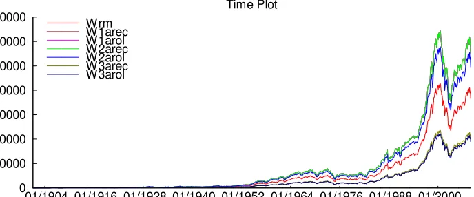
[image:16.612.154.471.397.542.2]0 200000 400000 600000 800000 1e+006 1.2e+006
01/1904 01/1916 01/1928 01/1940 01/1952 01/1964 01/1976 01/1988 01/2000 Time Plot
[image:17.612.155.483.130.278.2]Wrm W1arec W1arol W2arec W2arol W3arec W3arol
Figure 3: Cummulated Wealth from January 1901 to December 2007 for de-nominator B and forecasting models class A
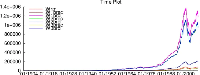
0 200000 400000 600000 800000 1e+006 1.2e+006 1.4e+006
01/1904 01/1916 01/1928 01/1940 01/1952 01/1964 01/1976 01/1988 01/2000 Time Plot
Wrm W1brec W1brol W2brec W2brol W3brec W3brol
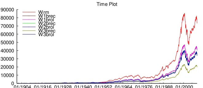
[image:17.612.153.480.359.482.2]0 10000 20000 30000 40000 50000 60000 70000 80000 90000
01/1904 01/1916 01/1928 01/1940 01/1952 01/1964 01/1976 01/1988 01/2000 Time Plot
[image:18.612.149.490.133.273.2]Wrm W1arec W1arol W2arec W2arol W3arec W3arol
Figure 5: Cummulated Wealth from January 1901 to December 2007 for de-nominator C and forecasting models class A
0 10000 20000 30000 40000 50000 60000 70000 80000 90000
01/1904 01/1916 01/1928 01/1940 01/1952 01/1964 01/1976 01/1988 01/2000 Time Plot
Wrm W1brec W1brol W2brec W2brol W3brec W3brol
[image:18.612.149.479.351.495.2]0 20000 40000 60000 80000 100000 120000 140000
01/1904 01/1916 01/1928 01/1940 01/1952 01/1964 01/1976 01/1988 01/2000 Time Plot
[image:19.612.162.506.131.274.2]Wrm W1arec W1arol W2arec W2arol W3arec W3arol
Figure 7: Cummulated Wealth from January 1901 to December 2007 for de-nominator D and forecasting models class A
0 20000 40000 60000 80000 100000 120000
01/1904 01/1916 01/1928 01/1940 01/1952 01/1964 01/1976 01/1988 01/2000 Time Plot
Wrm W1brec W1brol W2brec W2brol W3brec W3brol
[image:19.612.152.498.348.503.2]A.3
Test of Correlated Means
12 Months 24 Months 36 Months 48 Months 60 Months
Rtr > Rm 16 19 22 21 21
Rtr < Rm 20 20 20 20 20
[image:20.612.219.565.171.240.2]Rtr =Rm 12 9 6 7 7
Table 3:
The table summarizes the results from table 4 and de…nes the number of times one of the three di¤erent scenarios were witnessed. Rtr < Rmis the number of times that the accumulated return is higher than the trading rule. This proportion is a
litte high due to the adoption of denominator C,
Model 1a Rec 1a Rol 2a Rec 2a Rol 3a Rec 3a Rol 1b Rec 1b Rol 2b Rec 2b Rol 3b Rec 3b Rol 1 year:A -10.29 -10.43 -10.43 -10.27 2.81 0.18 -9.99 -9.99 -10.14 -10.14 2.22 -1.06
B -5.96 -5.56 -5.56 -6.05 2.76 0.58 -6.87 -6.87 -5.85 -5.92 3.22 -0.59 C 4.12 4.12 4.12 4.33 6.76 4.52 4.16 4.16 4.36 4.36 5.75 4.20 D -1.08 -1.08 -1.08 -0.25 3.79 3.97 0.53 0.53 0.53 0.53 3.79 3.59 2 year:A -14.33 -14.51 -14.51 -14.20 3.41 -0.25 -14.13 -14.13 -14.39 -14.39 2.75 -1.90
B -8.45 -7.97 -7.97 -8.71 3.63 0.34 -9.76 -9.76 -8.49 -8.56 4.43 -1.31 C 6.03 6.03 6.03 6.41 10.32 6.44 6.07 6.07 6.46 6.46 8.72 5.90 D -3.00 -3.00 -3.00 -1.36 5.57 5.36 0.08 0.08 0.09 0.08 5.57 4.84 3 year:A -18.67 -18.92 -18.92 -18.24 3.57 -1.00 -18.60 -18.60 -18.99 -18.99 2.97 -2.84
B -11.13 -10.65 -10.65 -11.69 4.03 -0.16 -12.94 -12.94 -11.43 -11.49 4.90 -2.07 C 7.26 7.26 7.26 7.86 12.36 7.59 7.31 7.31 7.91 7.91 10.35 6.94 D -4.53 -4.53 -4.53 -2.51 7.07 6.56 -0.45 -0.45 -0.44 -0.45 7.07 5.80 4 year:A -21.84 -22.08 -22.08 -21.03 4.07 -0.75 -21.87 -21.87 -22.33 -22.33 3.50 -2.60
B -12.19 -11.71 -11.71 -12.92 4.67 0.21 -14.46 -14.46 -12.77 -12.84 5.49 -1.66 C 8.14 8.14 8.14 8.73 13.31 8.41 8.19 8.19 8.78 8.78 11.27 7.81 D -4.45 -4.45 -4.45 -2.23 7.83 7.48 -0.16 -0.16 -0.15 -0.16 7.83 6.80 5 year:A -23.41 -23.63 -23.63 -22.58 3.87 -1.20 -24.16 -24.16 -24.28 -24.28 3.44 -3.13
B -13.66 -13.15 -13.15 -14.57 4.73 0.02 -16.36 -16.36 -14.49 -14.55 5.74 -1.90 C 8.40 8.40 8.40 9.21 14.62 9.25 8.45 8.45 9.26 9.26 12.43 8.56 D -5.97 -5.97 -5.97 -3.22 8.96 8.56 -0.85 -0.85 -0.84 -0.85 8.96 7.89
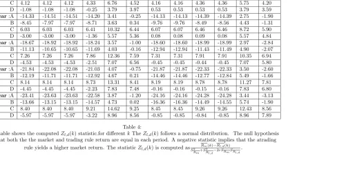
[image:21.612.111.671.133.403.2]Table 4:
The table shows the computedZl;d(k)statistic.for di¤erentkTheZl;d(k)follows a normal distribution. The null hypothesis
is that both the the market and trading rule return are equal in each period. A negative statistic implies that the atrading rule yields a higher market return. The statisticZl;d(k)is computed as
Rm(k) Rl;d(k)
S2
Rm+S
2
Rl;d 2rSRmSRl;d.
A.4
Sweeney X Statistic
One of the measures to account for the fact that wealth is held in both the stock market and in the bond market during the period of interest is given by the Sweeney(1989) statistic. The X statistic is given by:
X =Rtr (1 f)RBH
x= [f(1 f)=N] 1 2
1a Rec 1a Rol 2a Rec 2a Rol 3a Rec 3a Rol 1b Rec 1b Rol 2b Rec 2b Rol 3b Rec 3b Rol A 7.67 7.734 7.734 7.641 2.532 4.624 7.578 7.578 7.554 7.554 3.321 5.148 B 6.425 6.291 6.291 6.462 2.578 4.351 6.706 6.706 6.406 6.427 2.626 4.798 C 1.765 1.765 1.765 1.545 0.327 1.534 1.735 1.735 1.519 1.519 1.013 1.716 D 1.725 1.725 1.725 1.277 -0.382 -0.608 0.852 0.852 0.862 0.852 -0.382 -0.346
Table 5:
The table shows Sweeney’s statistic (X= x)over the whole sample period for the di¤erent models. Inference can be made
from the Normal distribution.
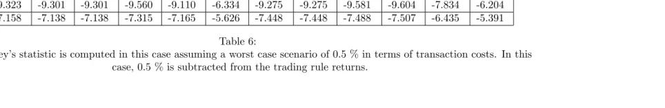
1a Rec 1a Rol 2a Rec 2a Rol 3a Rec 3a Rol 1b Rec 1b Rol 2b Rec 2b Rol 3b Rec 3b Rol A -2.603 -2.533 -2.533 -2.627 -6.781 -3.932 -2.669 -2.669 -2.705 -2.718 -5.704 -3.451 B -4.155 -4.289 -4.289 -4.091 -6.741 -4.154 -3.757 -3.757 -4.146 -4.142 -6.373 -3.714 C -9.323 -9.301 -9.301 -9.560 -9.110 -6.334 -9.275 -9.275 -9.581 -9.604 -7.834 -6.204 D -7.158 -7.138 -7.138 -7.315 -7.165 -5.626 -7.448 -7.448 -7.488 -7.507 -6.435 -5.391
Table 6:
The Sweeney’s statistic is computed in this case assuming a worst case scenario of 0.5 % in terms of transaction costs. In this case, 0.5 % is subtracted from the trading rule returns.
1a Rec 1a Rol 2a Rec 2a Rol 3a Rec 3a Rol 1b Rec 1b Rol 2b Rec 2b Rol 3b Rec 3b Rol A 5.466 5.525 5.525 5.525 0.487 2.810 5.367 5.367 5.354 5.351 1.287 3.293 B 3.914 3.769 3.769 3.769 0.528 2.588 4.280 4.280 3.912 3.927 0.618 3.030 C -1.254 -1.242 -1.242 -1.242 -1.842 0.408 -1.238 -1.238 -1.523 -1.534 -0.843 0.540 D 0.912 0.920 0.920 0.744 0.104 1.116 0.589 0.589 0.571 0.563 0.556 1.353
Table 7:
The Sweeney’s statistic is computed assuming a monthly rate of 0.25 % in terms of transaction costs.
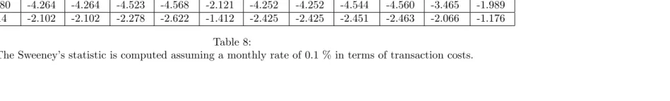
[image:23.612.108.657.273.351.2]1a Rec 1a Rol 2a Rec 2a Rol 3a Rec 3a Rol 1b Rec 1b Rol 2b Rec 2b Rol 3b Rec 3b Rol A 2.440 2.503 2.503 2.409 -2.238 0.282 2.354 2.354 2.332 2.325 -1.335 0.764 B 0.888 0.747 0.747 0.945 -2.198 0.060 1.266 1.266 0.890 0.901 -2.004 0.501 C -4.280 -4.264 -4.264 -4.523 -4.568 -2.121 -4.252 -4.252 -4.544 -4.560 -3.465 -1.989 D 2.114 -2.102 -2.102 -2.278 -2.622 -1.412 -2.425 -2.425 -2.451 -2.463 -2.066 -1.176
Table 8:
The Sweeney’s statistic is computed assuming a monthly rate of 0.1 % in terms of transaction costs.
A.5
Switching
A B C D
1a Recursive 883 857 884 1250
1a Rolling 881 858 884 1250
2a Recursive 881 858 884 1250
2a Rolling 884 858 883 1249
3a Recursive 882 881 874 1167
3a Rolling 766 774 863 1179
1b Recursive 885 863 886 1248
1b Rolling 885 863 886 1248
2b Recursive 890 860 884 1247
2b Rolling 890 859 884 1248
3b Recursive 817 823 847 1167
[image:25.612.216.396.154.334.2]3b Rolling 760 774 858 1190
Table 9:
The table illustrates the number of times that the rule postulates going long on the market in the di¤erent models. It is interesting to note that there is no
considerable di¤erence between denominator C as compared to the A and B. The worse performance may be due an improper timing.
A B C D
1a Recursive 420 402 42 10
1a Rolling 418 404 42 10
2a Recursive 418 404 42 10
2a Rolling 416 394 42 10
3a Recursive 92 78 40 10
3a Rolling 54 48 32 12
1b Recursive 422 392 42 10
1b Rolling 422 392 42 10
2b Recursive 412 392 42 12
2b Rolling 412 392 42 10
3b Recursive 102 82 34 10
3b Rolling 50 42 30 16
Table 10:
The table shows the number of times that the rule postulates switching assets in the case of the di¤erent models. Given the initial results previously, it may be noted that the models which has the highest accumulated wealth have more
[image:25.612.223.390.430.609.2]A.6
Tests on Forecasting Accuracy
AD test Kolgomorov Smirnov Doornik Hansen test
1a Recursive 20.82 0.09 690.13
1a Rolling 20.92 0.09 688.13
2a Recursive 20.92 0.09 688.13
2a Rolling 20.71 0.09 692.11
3a Recursive 6.08 0.05 3.73
3a Rolling 14.55 0.09 87.69
1b Recursive 12.63 0.07 456.59
1b Rolling 12.63 0.07 456.59
2b Recursive 13.36 0.06 469.29
2b Rolling 13.97 0.07 475.81
3b Recursive 3.88 0.04 4.13
[image:26.612.144.468.153.333.2]3b Rolling 14.11 0.9 113.27
Table 11:
The table does a test of normality of the forecasting error. The Anderson -Darling , Kolgomorov -Smirnov and Doornik Hansen test are reported. Most
of the tests show that the forecast errors are far from normal.
Model Sample Loss T-Statistic
MAE MSE MAE MSE MAE MSE
Most Signi…cant 2a Rol 2a Rol 0.065 0.009 -26.57 -10.6
Best 2a Rec 2a Rec 0.064 0.009 -26.6 -10.68
Model 25 % 2a Rol 2a Rol 0.065 0.009 -26.57 -10.6
Median 1b Rec 1b Rec 0.071 0.01 -29.4 -11.9
Model 75 % 3b Redc 3a Rec 1.758 4.59 -27.87 -19.51
Worst 3b Rol 3a Rol 2.967 5.84 -32.92 -13.98
Table 12:
The table shows the cummulated returns (in percentage) over the di¤erent periods: 1, 2, 3, 4 and 5 years for the di¤erent forecasting models and the
[image:26.612.149.468.416.533.2]A.7
Summary statistics
Dividends Log Dividends
Series Detrended Di¤erenced Series Detrended Di¤erenced
Mean 12.83 12.83 0.02 2.48 2.48 0.00
Std. Dev 4.66 2.27 0.13 0.37 0.20 0.01
Skewness 0.46 0.11 -0.48 -0.13 -0.59 -0.94
Kurtosis 2.50 2.71 7.12 2.00 2.71 10.25
Jarque-Bera 57.78 6.88 959.95 56.95 78.63 2996.31
ADF test -0.70 -1.27 -12.43 -0.86 -2.79 -12.12
PP test 1.04 -1.80 -18.34 -0.98 -2.89 -19.16
KPSS test 1.14 0.39 0.20 0.08 0.29 0.06
Lo’s Test 1.62 2.02 0.85 0.44 2.10 0.75
[image:27.612.134.513.154.323.2]Robinson’s d 0.49 0.50 0.34 0.50 0.50 0.31
Table 13:
A.8
Simulation Results
[image:28.612.125.664.161.349.2]12 Months 24 Months 36 Months 48 Months 60 Months Model A B C D A B C D A B C D A B C D A B C D 1a Recursive 67 55 23 5 93 79 34 12 104 91 38 16 119 101 36 21 127 101 36 21 1a Rolling 67 55 23 5 93 76 34 12 107 89 38 16 120 100 36 21 127 100 36 21 2a Recursive 67 55 23 5 93 76 34 12 107 89 38 16 120 100 36 21 127 100 36 21 2a Rolling 67 55 23 5 91 77 33 12 106 90 37 16 119 100 36 20 126 100 36 20 3a Recursive 37 37 14 6 41 42 24 10 44 45 25 10 46 45 22 8 50 45 22 8 3a Rolling 36 37 24 5 53 52 36 9 61 61 37 10 68 65 33 8 71 65 33 8 1b Recursive 67 55 23 5 93 76 34 11 102 92 38 15 118 101 34 17 127 101 34 17 1b Rolling 67 55 23 5 93 76 34 11 102 92 38 15 118 101 34 17 127 101 34 17 2b Recursive 69 53 23 5 92 77 33 11 100 91 37 15 118 100 34 17 127 100 34 17 2b Rolling 69 53 23 5 92 77 33 11 100 91 37 15 118 100 34 17 127 100 34 17 3b Recursive 39 35 21 6 46 39 30 10 54 43 30 10 56 48 29 8 61 48 29 8 3b Rolling 39 39 26 5 57 56 38 9 64 62 42 10 70 65 37 8 75 65 37 8
Table 14:
The table illustrates the number of times, the rule strictly beats the Passive Buy and Hold strategy for the respective forecasting model and denominator The simulation was attempted 160 times.
A.9
Fama and French’s Expected Returns
TheFama and French (2002)factors assume that if Price and Dividends are
cointegrated, the sum of the dividend price ratio and dividend growth would yield expected returns measures. The ADF test on the residual term in the dividend and price relationship was -4.10 while that with earnings and price was -4.33.
For real time purposes, tested for the stationarity of D P and
E
P using both
rolling and recursive ADF tests. The results tend to di¤er as to which criterion is used to select the residual term in the ADF equation. The various criteria used are Akaike Information Criteria, Bayesian Information Criteria, Schwartz Information Critera, Hannan Quinn and the Modi…ed Information criteria. We report the Bayesian Information Criteria. (The other plots are available upon request)
-5 -4.5 -4 -3.5 -3 -2.5 -2 -1.5 -1 -0.5 0 0.5
01/1904 01/1916 01/1928 01/1940 01/1952 01/1964 01/1976 01/1988 01/2000 Time Plot
[image:29.612.179.436.341.467.2]T-stat(BIC) 1% 5% 10%
Figure 9: Recursive ADF T-stat (BIC optimal Lag selection) for the Dt
Pt:
-5 -4 -3 -2 -1 0 1 2
01/1904 01/1916 01/1928 01/1940 01/1952 01/1964 01/1976 01/1988 01/2000 Time Plot
T-stat(BIC) 1% 5% 10%
Figure 10: Recursive ADF T-stat (BIC optimal lag selection) for Et
[image:29.612.175.438.524.629.2]