Federal, State, and Local Governments: Evaluating their Separate Roles in US Growth

Federal, State, and Local Governments:

Evaluating their Separate Roles in US

Growth

Higgins, Matthew and Young, Andrew and Levy, Daniel

Georgia Institute of Technology„ University of Mississippi, and,

Bar-Ilan University

29 January 2009

Online at

https://mpra.ub.uni-muenchen.de/13094/

Matthew J. Higgins

College of Management, Georgia Institute of Technology

Andrew T. Young**

Department of Economics, University of Mississippi

Daniel Levy

Department of Economics, Bar-Ilan University, Department of Economics, Emory University, and

Rimini Center for Economic Analysis

Last Revision: January 2009

Abstract We use US county level data (3,058 observations) from 1970 to 1998 to explore the relationship between economic growth and the extent of government employment at three levels: federal, state and local. We find that increases in federal, state and local government employments are all negatively associated with economic growth. We find no evidence that government is more efficient at lower levels. While we cannot separate out the productive and redistributive services of government, we document that the county-level income distribution became slightly more unequal from 1970 to 1998. For those who justify government activities in terms of equity concerns – perhaps even trading off economic growth for equity – the burden falls on them to show that the income distribution would have widened more in the absence of government activities. We conclude that a release of government-employed labor inputs to the private sector would be growth-enhancing.

JEL Codes O40 O11 O18 O51 R11 H50 H70

Key Words Economic Growth, Federal Government, State Government, Local Government, and County-Level Data

**

1 Introduction

Does government contribute to or hinder economic growth? This question is of

considerable interest to economists and is the subject of a large empirical literature.

However, government is a very broad concept. A more appropriate and tractable question

is: what kinds of government contribute to or hinder economic growth? To address this

question, we revisit and extend a number of results from Higgins et al.’s (2006) study of

United States growth determination. In that paper we use county-level data to assess the

roles of federal, state, and local government, separately, in growth determination from

1970 to 1998. The analysis focuses on levels of centralization as the relevant kinds of

government. Nearly all of the evidence that we present in Higgins et al. (2006) suggests

that government, at any level, hinders economic growth. Furthermore, there is no

evidence that government's negative effect on growth diminishes at lower levels.

In this paper we report how the basic Higgins et al. (2006) findings are largely

robust to examining (a) subsamples of metro and non-metro counties separately, (b)

regional subsamples, and (c) individual US state subsamples. We also (d) employ a more

careful selection of valid instruments for our regressions. The basic findings are again

robust. We also include documentation that (e) the county-level income distribution

widened slightly over the 1970 to 1998 period.

Our 2006 paper primarily focuses on conditional convergence rates in the United

States. Determinants of balanced growth paths are given second-order treatment in terms

of detail and space. This paper allows us to highlight findings associated with the role of

government employment variables in growth determination. We believe that the focus on

through (e) provides a stronger and more thorough argument that government activities

are growth-retarding in the United States.

The paper is organized as follows. Section 2 elaborates on the questions of

interest in terms of the existing literature and how we add to that literature. Section 3 then

briefly discusses the econometric method and data that we employ. Section 4 discusses

the empirical findings. Concluding remarks are made in Section 5.

2 Growth and Government: The Existing Literature

When asking about kinds of United States government there are two

complementary (and not mutually exclusive) categorizations of interest. One

categorization is kinds of government services and inputs to production and has received

considerable attention in the literature. A seminal example is Aschauer (1989) who

analyzes government military and non-military investment, finding that only non-military

government investment is positively associated with state-level economic growth.

Alternatively, Holtz-Eakin (1994) finds that government investment has a negative effect

or no effect on gross state product (GSP) growth. Evans and Karras (1994) confirm the

Holtz-Eakin result even when considering investments in highways, water and sewer

capital, and other infrastructure capital separately.1 However, Evans and Karras also find

that increases in government educational services are positively related to growth.2 A

more recent paper by Shioji (2001) revisits the effects of different types of government

1

Garcia-Milà et al. (1996) confirm these results. Lynde and Richmond (1993), to the contrary, use a translog production function specification and find that government investment contributes to output growth while the government capital stock contributes to productivity growth.

2

investment. He finds that the infrastructure component has a positive effect on growth.3

This literature, thus, offers mixed evidence.

The categorization we explore – namely kinds of government in terms of the level

of decentralization – has not received as much attention in the literature. In a sample of

58 countries, an early paper by Oates (1972) finds that measures of fiscal decentralization

(henceforth simply decentralization) positively correlate with real income per capita.4

Davoodi and Zou (1998), on the other hand, find that decentralization is negatively

associated with growth in developing countries, and not associated with growth in

developed countries.

The literature is especially sparse in regards to the United States economy.5 Three

notable exceptions are Xie et al. (1999) who fail to find a relationship between

decentralization and per capita income growth from 1948 to 1994 and Akai and Sakata

(2002) and Stansel (2005) who find positive relationships between decentralization and

growth.6 Xie et al. (1999) focus on the share of local and state government in aggregate

government expenditures. Akai and Sakata (2002) analyze expenditure and revenue

shares of federal, state and local governments in state-level cross-section data. Finally,

3

Different kinds of government services and inputs to production are also a common focus of cross-country studies. Examples include Atkinson (1995), Slemrod (1995), Agel et al. (1997), Sala-i-Martin (1997a, 1997b), and Baldacci et al. (2004).

4

Despite Oates' (1972) empirical finding, the relationship between economic growth and fiscal

decentralization in general cannot be directly linked to the more specific “decentralization theorem” put forth by Oates in the same work. The decentralization theorem concerns the welfare advantages of localized public goods provision in the absence of “cost-savings from centralized provision” and “interjurisdictional externalities” (p. 72). The theorem only establishes “a presumption in favor of the decentralized provision of public goods with localized effects” (Oates, 1999, p. 1122). Difficult questions involve, first, whether this implies a presumption that decentralization positively correlates with growth and, second, whether the assumptions underlying that presumption actually hold in a given economy.

5

Studies specific to countries other than the United States include Carrion-i-Silvestre et al. (2008) for Spain and Zhang and Zhou (1998) for China.

6

Stansel (2005) examines the central city share of population, per capita municipalities,

and per capita counties.

Our analysis complements the above studies. We focus on federal, state, and local

government employment as a percentage of a county's population. Our analysis of

employment shares is novel in terms of both (i) the underlying concept of the public

sector (or the dimensions of the public sector measured) and (ii) the economic unit of

analysis (i.e., a county). Employment shares come from the county-level data that

Higgins et al. (2006, 2008) and Young et al. (2008) exploit to study convergence in the

United States. In contrast to the 48-to-50 state-level observations, or the 314 metropolitan

areas studied by Stansel (2005), our data contain over 3,000 county-level observations.

Employment shares may provide a better measure of many government activities

than expenditure shares do. They capture percentages of available labor input that are

being directed by a specific level of the public sector (rather than by the decisions of

private individuals and firms). To the extent that economically important government

activities are labor-intensive, analyzing the effects of employment shares is of interest.

For example, regulatory environments are presumably inherently labor-intensive in that

they are not effective without investigative monitoring and enforcement on the ground.7

Moreover, the large number of cross-sectional observations allows us to study the

United States as a whole as well as various sub-samples of interest. Metro and non-metro

sub-samples allow for the possibility that government's effect on economic growth varies

with population density and provides a link to the metro area study of Stansel (2005).

7

There are, of course, also advantages to expenditure shares relative to employment shares. For

For instance, a higher population density may lead to negative externalities that the public

sector is uniquely suited to deal with. Furthermore, regional and individual state samples

(the latter of which Higgins et al. (2006, 2008) do not explore) allow for the possibility of

heterogeneity of institutions and cultures that are conducive to, or foster, relatively good

or bad government (in terms of growth-determination). For example, the general view of

what activities government should pursue may be very different in different regions of

the country. This carries over to the federal level if individual states request, allow,

and/or encourage different types of federal activities. In that case, the effects of

government on growth may be significantly different.

Our analysis incorporates 38 variables (as well as state-dummies for the

nation-wide samples) on which to condition the growth rates of per capita income. These

variables control for the effects of various levels of educational attainment, age, racial

demographics, and industry composition.

Following Higgins et al. (2006), we use a cross-sectional variant of the 3SLS-IV

approach of Evans (1997). However, we improve upon Higgins et al. (2006) in terms of

the instruments used. Higgins et al. (2006) employed lagged values of all conditioning

variables as instruments. We employ an algorithm that chooses from those lagged values

a set of instruments that (i) are valid and (ii) have the highest Shea partial R2.

3 Empirical specification and data

In this section we briefly describe the basic growth regression model and the estimation

Finally, since our estimation technique employs instrumental variables, we describe the

algorithm that we use to optimally choose a set of instruments conditional on the

available data.

3.1 The regression model and 3SLS-IV estimation procedure

Our growth regressions involve fitting cross-sectional data to the equation,

(1) g_n =α+βy_n0 +γ′x_n +ν_n,

where g_n is the average growth rate of per capita income for economy n between years 0

and T; yn0 is initial (t = 0) per capita income; xn is a vector of other control variables

including government employment shares; and γ are coefficients; and νn is a zero

mean, finite variance error term.8 Given our data, 0 1970 and T 1998.9

Caselli, et al. (1996) and Evans (1997) show that applying OLS to (1) will yield

consistent estimates only if the data satisfy highly implausible conditions.10 Evans (1997)

proposes a 3SLS-IV method that produces consistent estimates. In the first two stages,

instrumental variables are used to estimate the regression equation,

(2) ∆g_n =ω +β∆y_n0 +η_n,

where

T y y

T y y

g_n = ( n,T − n,0)−( n,T−1 − n,−1)

∆ , ∆y_n0 = y_n0 − y_n,−1, y_n , ω is a parameter,

8

For a derivation of this regression from a neoclassical growth model, see Barro and Sala-i-Martin (1992). For exposition of this model in greater detail see Higgins et al. (2006).

9

Though the period of growth under consideration is 28 years, the analysis is essentially cross-sectional because average growth over those 28 years is the single dependent variable.

10

and η_n is the error.11 ,12

Next, we useβ*, the estimate from (2), to construct the variable,

(3) πn =gn −β*yn₀.

In the third stage, we perform an OLS regression ofπ_n on x_n:

(4) π_n =τ +γx_n +ε_n,

where and are parameters and n is the error term. This regression yields a consistent

estimator, *.

3.2 US county-level data

The data we use are drawn from several sources but the majority comes from the

Bureau of Economic Analysis Regional Economic Information System (BEA-REIS) and

United States Census data sets. The BEA-REIS data are largely based on the 1970, 1980

and 1990 decennial Census files; the 1972, 1977, 1982 and 1987 Census of Governments;

and the Census Bureau’s City and County Book from various years. We exclude military

personnel from all data.

11

An immediate concern with the use of (2) is the reliance on the information from the single difference in the level of income (1969 to 1970) to explain the difference in average growth rates over overlapping time periods (1969 to 1997 and 1970 to 1998). Given that the growth determination is a stochastic process, the potential problem is basically one of a high noise to signal ratio. We are relying on large degrees of freedom to alleviate this problem and identify coefficients. Indeed, we obtain statistically significant estimates for the full sample as well as for 32 individual states.

12

As Evans (1997) shows, the derivation of this equation depends on the assumption that the xn variables

Our data contain 3,058 county-level observations. The large number of

observations allows us to explore possible heterogeneity in growth across the United

States by splitting the data into three sets of subsamples. The first set includes a metro

subsample (867 counties) and a non-metro subsample (2,191 counties).13 The second set

includes 5 regional subsamples: Great Lakes, Northeast, Southern, Plains, and Western.

Finally, the third set includes 50 individual US state subsamples.

We use the BEA’s measure of personal income net of government transfers

expressed in 1992 dollars. Natural logs of real per capita income are used throughout.

The 38 conditioning variables are the same as in Higgins et al. (2006, Table 1) and

account for various age and racial demographics, levels of educational attainment, and

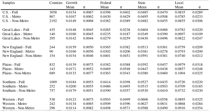
industry employment composition.14 For the variables of interest to the present analysis,

Table 1 reports some summary statistics for the various samples of United States

counties. The variables are average per capita income growth rates from 1970 to 1998

and federal, state, and local government employments as percentages of a county's

population.

3.3 Choice of Instruments

Higgins et al. (2006) used lagged values of conditioning variables as instruments

for yn,0 in equation (2). A basic criticism of that paper is that no evidence was presented

of those instruments' validity. It is well-known that a valid set of instruments includes

variables that are correlated with the endogenous regressors (instrument relevance) but

13

Metro counties are defined as those that contain cities with populations of 100,000 or more, or border such counties (Higgins et al. 2006)

14

uncorrelated with the error term of the regression (instrument orthogonality). For a given

set of instruments, an F-statistic test can be used to assess the former while

overidentification tests can be used to assess the latter.

In the case of a single endogenous regressor, such as the case with yn,0 in

equation (2), Staiger and Stock (1997) have suggested declaring instruments to be weak

(not relevant) if the first-stage F-statistic is less than ten (Stock and Yogo 2002). This

“rule of thumb” for testing instrument relevance is supported by Baum et al. (2003). In

regard to instrument orthogonality, Deaton (1997) and Stock and Yogo (2002) point out

that when several instruments are used, overidentification tests can be applied. In the

present case we use Sargan’s (1964) overidentification test to assess whether the

instruments are correlated with the error process.15

Given the size of our sample and the number of independent variables, we have a

large number of potential instruments. In order to generate a set of valid instruments, i.e,

those that address instrument relevance and orthogonality, we apply an algorithm that (i)

selects various combinations of available (lagged) conditioning variables such that the

system is overidentified, (ii) tests their validity and, (iii) if found valid, uses them in the

regression analysis. Our algorithm does not maximize any particular function but rather

aids in sifting through all various combinations of valid instruments (i.e., those where the

first-stage F-statistic is greater than 10 and that pass the Sargan test). From this subset of

valid instruments we selected the set that produced the largest first-stage Shea (1997)

partial R2, 0.3510.

Our final set of instruments consists of the following 13 lagged variables: “Age:

18-64 years”, “Education: Bachelor +”, “Federal government employment”, “State

15

government employment”, “Local government employment”, “Self-employment”,

“Agriculture”, “Construction”, “Manufacturing: durables”, “Manufacturing:

non-durables”, “Health services”, “Personal services”, and “Entertainment & Recreational

Services”.16

4 Empirical findings

We begin by presenting our empirical estimates of the effect of federal, state, and local

government employment (as a percentage of a county's population), separately, on United

States economic growth at the county-level. Estimates are presented for (a) country-wide

samples, including metro and non-metro subsamples, (b) regional subsamples, and (c)

individual state subsamples. We also informally consider the redistributive role of

government which may account for the lack of positive growth effects of government

employment.

4.1 Full US sample results

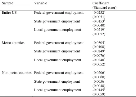
Table 2 presents the estimation results for the full United States sample, as well as

metro and non-metro samples. We find a negative and statistically significant partial

correlation between the percentage of the population employed by government and the

rate of economic growth, regardless of whether one considers federal, state or local

government. The coefficients for federal, state and local government employment

16

percentages of the population variables are –0.0252, –0.0153, and –0.0219 respectively,

all significant at the 1% level. There is no clear pattern in the point estimates as the level

of decentralization increases, and the 95% confidence intervals of the point estimates are

overlapping.17

The negative effects are also present at all levels of government employment

whether one considers only metro counties or only non-metro counties as indicated by the

figures in Table 2. This suggests that government employment is not positively related to

economic growth at higher population densities. Indeed the negative partial correlations

are larger for the metro sample than for the non-metro sample at all levels.

Given the apparent robustness of a negative association between government

employment with growth, one interpretation is that federal, state and local government

activities misallocate resources into relatively (compared to the private sector) inferior

production processes. Government lowers total factor productivity, thus lowering

balanced growth paths. However, another interpretation may be entertained. Perhaps

non-government wage growth outpaces non-government wage growth, and this drives the

results.18 These interpretations are not incompatible in a world where both government

and non-government wages approximate marginal products. However, government

employment, not being subject to the same market forces, may be different along certain

17

The relationship may, however, be nonlinear. Government expansion may promote growth but only up to a point when further expansion is detrimental to growth at the margin; or it may be the case that

government expansion aims to enhance growth up to a point, and then expansion beyond that point aims at income redistribution (Buchanan and Wagner 1977). To check this, we run the full US sample regression including both linear and quadratic government employment share terms. Only for the federal employment share is the quadratic term positive and significant, but the parameter estimates imply that the marginal effect is negative up until the federal government employs over 30% of a county's population; the total effect is negative until it employs over 60%! (In the data, however, only nine out of 3,058 counties have a federal government employment share in excess of 30%.)

18

intangible margins (e.g., greater job security; lower expectations of effort; higher psychic

benefits associated with providing a public service).

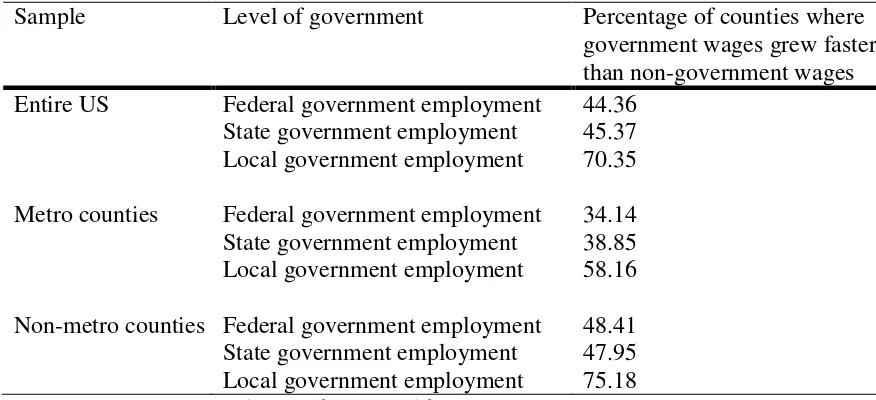
In order to explore the above we have assembled government and

non-government wage growth data for the sample period (Table 3). At the state and federal

level, non-government wages outpace government wages in approximately 55% (a small

majority) of all counties. At the local level, non-government wages grew faster in only

about 30% of counties. Relative sluggishness of government wages at the state and

federal levels is dominated by wage growth rates in the metro counties. For the

non-metro counties, which constitute a vast majority of 2,196 counties panel, non-government

wages outpaced government wages in just over 50% of cases.19

If a relatively sluggish growth of government wages story were important, then

we would expect to find smaller estimated coefficients for metro counties than for

non-metro counties. This we do see. The coefficient estimates for the regression including

only metro counties are –0.0300, –0.0264 and –0.0214 for federal, state and local

governments respectively. For non-metro counties the corresponding estimates are –

0.0179, –0.0081 and –0.0128. Note, however, that this pattern holds for the local

government coefficients as well, despite local wages outpacing non-government wages in

a majority of counties. At least at the most decentralized level of government, a relatively

sluggish government wage growth story is unable to account for the negative partial

correlation. Indeed, we find a negative relationship despite the relatively fast growth of

government wages.

19

4.2 Regional Results and Individual State Results

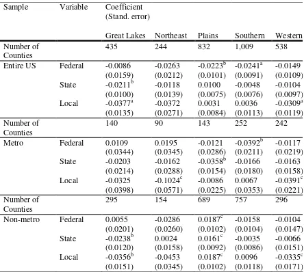
Table 4 reports the results for our five regional sub-samples: Great Lakes,

Northeastern, Southern, Plains and Western. Statistically significant results are harder to

come by using these smaller samples, but those significant coefficient estimates are

broadly consistent with our full sample findings. The significant coefficient estimates are

all negative except for those associated with the metro Plains region. For the

non-metro Plains region, notably, positive effects are estimated for all levels of government.

The statistically significant coefficient estimates that are negative occur, variously, for

federal, state, and local government.20

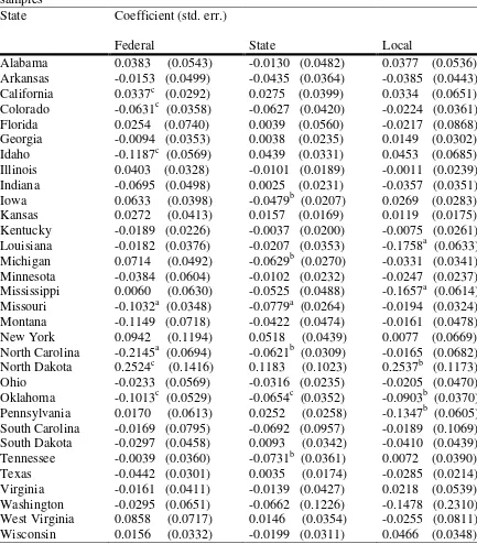
Table 5 reports the estimates for 32 of 50 individual US state sub-samples.21

Again, these results are broadly consistent with the conclusion that government

employment, at all levels, is negatively correlated with economic growth. Almost all

statistically significant effects are negative. The notable exception is North Dakota. North

Dakota has large, statistically significant positive coefficients on federal and local

government employment.

It is not immediately apparent what might be peculiar about North Dakota. For

example, in 1970, North Dakota ranked 21st highest in terms of federal government

employment (1.3%); 7th in terms of state government employment (2.3%); and 4th in

terms of local government employment (4.7%). However, similar to the Plains region

20

The non-metro Plains region effects may be associated with relatively fast government wage growth. Federal, state, and local government wage growth, respectively, outpaced non-government wage growth in approximately 62%, 68%, and 80.32% of counties.

21

metro case, federal, state, and local government wage growth was higher than

non-government wage growth in, respectively, about 57%, 75%, and 85% of counties. This

exceptional government relative wage growth may account for the estimated positive

effect of government employment on income growth.22

4.3 Redistributive Activities

It is possible that the negative correlation between government employment and

economic growth is due to the redistributive activities of government. Redistributive

activities may be detrimental towards average (per capita) income growth though

effective in their specific goals. Furthermore, if greater income equality is valued in and

of itself, then trading off growth for equity may be viewed as desirable.

Our analysis cannot separate out the productive and redistributive activities of

federal, state, or local governments. However, under the hypothesis that the negative

correlation between government employment and economic growth is due to

redistributive activities, we can ask whether or not economic growth has indeed been

traded off for a more equitable distribution of income. In other words, we can evaluate a

possible redistributive role for the various levels of government given the caveat that we

cannot control for how the distribution of income might have evolved in the absence of

government. (Clearly this caveat is an important one.)

Young et al. (2008) provide evidence on this issue; here we briefly summarize

their results. Figure 1 displays the 1970 and 1998 distributions of per capita income

across US states. The distribution became more unequal. Also, the Gini coefficients

22

associated with United States counties' 1970 and 1998 (log) incomes are 0.0167 and

0.0165 respectively – a decrease of about 1.2%.23 At the county-level, the dispersion of

United States per capita income became more unequal from 1970 to 1998.24 However,

changes in both the standard deviation and the Gini coefficient are small enough to

suggest that changes in both dispersion and equality are negligible.

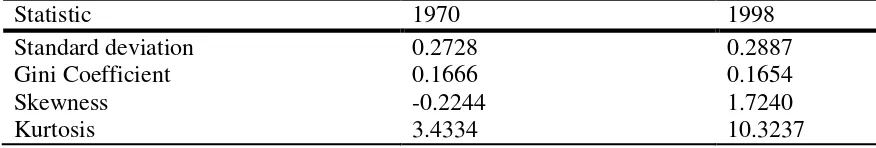
To try to understand further the evolution of the United States county-level

income distribution, Table 6 summarizes statistics computed from the 1970 and 1998

income distributions. From 1970 to 1998, the skewness of the distribution increased from

-0.2244 (to the left) to 1.7240 (to the right). At the same time, kurtosis increased from

3.4334 to 10.3237, implying that the distribution has become more peaked. Cumulatively,

this suggests that these two effects have been offsetting to a great extent.

In conclusion, the evidence presented in Young et al. (2008) does not suggest that

government activities have achieved (absolutely) a more equal distribution of income at

the expense of lower rates of economic growth. Put differently, it suggests government

failure at federal, state, and local levels in lieu of evidence that the distribution of

county-level per capita income would have widened significantly in the absence of government

activities.

5 Concluding Remarks

We use United States county data containing over 3,000 cross-sectional observations

during the period 1970 to 1998 to explore the relationships between economic growth

23

The Gini coefficient is a number between 0 (perfect equality) and 1 (perfect inequality).

24

and the size and scope of government at three levels: federal, state and local. In contrast

to the extant literature that has used taxes, government expenditures and government

capital stocks to proxy for the extent of government, here we focus on government

employment shares.

Following Higgins, et al. (2006), we use a 3SLS-IV estimation technique and

report on the full sample of United States counties, as well as metro and non-metro

subsamples, and five regional and 32 individual state subsamples. We find that federal,

state and local government employment shares almost always negatively correlate with

growth (when statistical significance holds) across samples.

We find no evidence that government is more effective at more or less

decentralized levels. Furthermore, while we cannot separate out the productive and

redistributive services of government, we document that income inequality in the United

States has widened slightly from 1970 to1998. However, the change in both the standard

deviation of per capita income and the Gini coefficient are small enough to suggest that

both dispersion and equality remained essentially the same.

Given the ostensible goals of higher growth and/or a more equitable distribution

of income, our findings are not supportive of expanding the roles of government, in terms

of employment, at any level. While government is often invoked as a solution to market

failures, the evidence points to government failure as a more important, and negative,

influence in the economy. Our findings suggest a rolling back of government activities;

specifically for a release of government-employed labor inputs to the private sector.

The most important and obvious caveat to our findings is that we cannot

infrastructure development. Despite examining federal, state, and local government

separately, we must view each level of government as a given package of activities and

services. Still, our results are consistent with the conclusion that, as currently composed,

a shrinking of government at any and all levels of decentralization would be a desirable

policy.

Acknowledgements We are grateful to the anonymous referee for constructive comments and suggestions,

and to an associate editor and the editor for advice. We thank the participants at the 2006 APEE meetings

for helpful comments and suggestions. We also thank Jordan Rappaport for kindly sharing with us his data

and computer codes from Rappaport (1999), and Arye Hillman, Paul Rubin, and Avichai Snir for

discussions. Daniel Levy gratefully acknowledges financial support from Adar Foundation of the

Economics Department at Bar-Ilan University. Higgins gratefully acknowledges financial support from The

References

Agel, J., Lindh, T., & Ohlsson, H. (1997). Growth and the public sector: a critical review

essay. European Journal of Political Economy, 13 (1), 33-52.

Akai, N., & Sakata, M. (2002). Fiscal decentralization contributes to economic growth.

Journal of Urban Economics, 52 (1), 93-108.

Aschauer, D. A. (1989). Is public expenditure productive? Journal of Monetary Economics,

24 (2), 177-200.

Atkinson, A. B. (1995). The welfare state and economic performance. National Tax

Journal, 48 (2), 171-198.

Baldacci, E., Hillman, A., & Kojo, N. (2004). Growth, governance, and fiscal policy

transmission channels in low-income countries. European Journal of Political

Economy, 20 (3), 517-549.

Barro, R. J., & Sala-i-Martin, X. (1992). Convergence. Journal of Political Economy, 100

(2), 223–251.

Baum, C.F., Schaffer, M.E., & Stillman, S. (2003). Instrumental variables GMM:

estimation and testing. The Stata Journal, 3 (1), 1-31.

Brueckner, J. (2006). Fiscal federalism and economic growth. Journal of Public

Economics, 90 (10-11), 2107-2120.

Buchanan, J., & Wagner, R. (1977). Democracy in deficit: the political legacy of lord

Keynes. New York: Academic Press.

Caselli, F., Esquivel, G., & Lefort, F. (1996). Reopening the convergence debate: a new

363–390.

Carrion-i-Silvestri, J. L., Espasa, M., & Mora, T. (2008). Fiscal decentralization and

economic growth in Spain. Public Finance Review, 36 (2), 194-218.

Davoodi, H., & Zou, H. (1998). Fiscal decentralization and economic growth: a cross-

county study. Journal of Urban Economics, 43 (2), 244-257.

Deaton, A., (1997). The analysis of household surveys: microeconomic approach to

development policy. Baltimore: Johns Hopkins University Press.

Evans, P., (1997). Consistent estimation of growth regressions (Manuscript).

http://economics.sbs.ohiostate.edu/pevans/pevans.html.

Evans, P. & Karras, G. (1994). Are government activities productive? evidence from a

panel of US states. Review of Economics and Statistics, 76 (1), 1–11.

Garcia-Milà, T., McGuire, T. J., & Porter, R. H. (1996). The effect on public capital in

state-level production functions reconsidered. Review of Economics and Statistics,

78 (1), 177-180.

Higgins, M. J., Levy, D., & Young, A. T. (2006). Growth and convergence across the US:

evidence from county-level data. Review of Economics and Statistics,

88 (4), 671-681.

Higgins, M. J., Young, A. T., & Levy, D. (2009). Robust correlates of US county-level

growth. Applied Economics Letters, (Forthcoming).

Hillman, A. (2003). Public finance and public policy: responsibilities and limitations of

government. New York: Cambridge University Press.

Holtz-Eakin, D. (1994). Public-sector capital and the productivity puzzle. Review of

Lynde, C., & Richmond, J. (1993). Public capital and total factor productivity.

International Economic Review, 34 (2), 401-413.

Martinez-Vazquez, J. and McNab, R. M. (2003). Fiscal decentralization and economic

growth. World Development, 31 (9), 1597-1616.

Oates, W. E. (1972). Fiscal federalism. New York: Harcourt Brace Jovanovic.

Oates, W. E. (1999). An essay on fiscal federalism. Journal of Economic Literature, 37

(3), 1120-1149.

Rappaport, J. (1999). Local growth empirics. CID Working Paper #23, Harvard University.

Rappaport, J. (2005). How does labor mobility affect income convergence?

Journal of Economic Dynamics and Control, 29 (3), 567-581.

Rappaport, J., & Sachs, J. D. (2003). The United States as a coastal nation. Journal of

Economic Growth, 8 (1), 5–46.

Sala-i-Martin, X. (1997a). I just ran two million regressions. American Economic Review,

87 (2), 178-193.

Sala-i-Martin, X. (1997b). I just ran four million regressions. NBER Working Paper No.

6252.

Sargan, D. (1964). Wages and prices in the United Kingdom: a study in econometric

methodology. In Econometrics analysis for national economic planning. London:

Butterworths.

Shea, J. (1997). Instrument relevance in multivariate linear models: a simple measure.

Review of Economics and Statistics, 79 (1), 348 – 352.

Shioji, E. (2001). Public capital and economic growth: a convergence approach. Journal of

Slemrod, J. (1995). What do cross-country studies teach us about government

involvement, prosperity, and economic growth. Brookings Papers on Economic

Activity, 26 (2), 373–431.

Staiger, D., & Stock, J. H. (1997). Instrumental variables regression with weak

instruments. Econometrica, 65 (3), 557–586.

Stansel, D. (2005). Local decentralization and local economic growth: a cross-sectional

examination of US metropolitan areas. Journal of Urban Economics, 57 (1),

55-72.

Stock, J.H., & Yogo, M. (2002). Testing for weak instruments in linear regression. In

Identification and Inference in Econometric Models: Essays in Honor of Thomas J.

Rothenberg. Cambridge: Cambridge University Press.

Wooldridge, J. (2001). Econometric Analysis of Cross Section and Panel Data. Boston:

The MIT Press.

Xie, D., Zou, H., & Davoodi, H. (1999). Fiscal decentralization and economic growth in

the United States. Journal of Urban Economics, 45 (2), 228-239.

Young, A. T., Higgins, M. J., & Levy, D. (2009). Sigma convergence versus beta

convergence. Journal of Money, Credit, and Banking, 40 (5), 1083-1094.

Zhang, T. & Zou, H. (1998). Fiscal decentralization, public spending, and economic growth

Samples Counties Growth Federal State Local

Mean Mean Mean Mean

U.S. - Full 3058 0.0154 0.0067 0.0396 0.0402 0.0485 0.0470 0.0835 0.0289

U.S. - Metro 867 0.0167 0.0062 0.0430 0.0429 0.0495 0.0508 0.0785 0.0233

U.S. - Non-Metro 2192 0.0149 0.0068 0.0382 0.0389 0.0482 0.0455 0.0855 0.0306

Great Lakes - Full 435 0.0148 0.0045 0.0265 0.0238 0.0404 0.0466 0.0782 0.0220

Great Lakes - Metro 140 0.0160 0.0045 0.0235 0.0187 0.0349 0.0390 0.0697 0.0109

Great Lakes - Non-Metro 295 0.0142 0.0044 0.0279 0.0259 0.0430 0.0496 0.0822 0.0247

New England - Full 244 0.0159 0.0050 0.0365 0.0382 0.0513 0.0361 0.0759 0.0209

New England - Metro 90 0.0166 0.0056 0.0302 0.0206 0.0381 0.0278 0.0793 0.0200

New England - Non-Metro 154 0.0154 0.0046 0.0401 0.0451 0.0591 0.0381 0.0740 0.0212

Plains - Full 832 0.0139 0.0075 0.0382 0.0388 0.0392 0.0457 0.0979 0.0318

Plains - Metro 143 0.0171 0.0052 0.0469 0.0548 0.0447 0.0438 0.0857 0.0248

Plains - Non-Metro 689 0.0133 0.0077 0.0363 0.0343 0.0380 0.0460 0.1004 0.0325

Southern - Full 1009 0.0184 0.0053 0.0414 0.0398 0.0527 0.0435 0.0726 0.0220

Southern - Metro 252 0.0200 0.0055 0.0486 0.0495 0.0515 0.0503 0.0709 0.0185

Southern - Non-Metro 757 0.0179 0.0051 0.0390 0.0357 0.0530 0.0410 0.0732 0.0230

Western - Full 538 0.0123 0.0075 0.0503 0.0499 0.0606 0.0558 0.0895 0.0325

Western - Metro 242 0.0134 0.0065 0.0509 0.0396 0.0627 0.0631 0.0868 0.0284

Western - Non-Metro 296 0.0114 0.0082 0.0498 0.0571 0.0588 0.0490 0.0916 0.0354

Table 2 Estimated effects of government employment on growth: US-wide samples

Sample Variable Coefficient

(Standard error)

Entire US Federal government employment -0.0252a

(0.0051)

State government employment -0.0153a

(0.0040)

Local government employment -0.0219a

(0.0052)

Metro counties Federal government employment -0.0305a

(0.0108)

State government employment -0.0249a

(0.0076)

Local government employment -0.0240a

(0.0052)

Non-metro counties Federal government employment -0.0206a

(0.0060)

State government employment -0.0056

(0.0048)

Local government employment -0.0145a

TABLES (Cont.)

Table 3 Estimated effects of government employment on growth: US-wide samples

Sample Level of government Percentage of counties where

government wages grew faster than non-government wages

Entire US Federal government employment 44.36

State government employment 45.37

Local government employment 70.35

Metro counties Federal government employment 34.14

State government employment 38.85

Local government employment 58.16

Non-metro counties Federal government employment 48.41

State government employment 47.95

Local government employment 75.18

Table 4 Estimated effects of government employment on growth: US regional samples

Sample Variable Coefficient

(Stand. error)

Great Lakes Northeast Plains Southern Western

Number of Counties

435 244 832 1,009 538

Entire US Federal -0.0086

(0.0159) -0.0263 (0.0212) -0.0223b (0.0101) -0.0241a (0.0091) -0.0149 (0.0109)

State -0.0211b

(0.0100) -0.0118 (0.0139) 0.0100 (0.0075) -0.0048 (0.0076) -0.0104 (0.0097)

Local -0.0377a

(0.0135) -0.0372 (0.0271) 0.0031 (0.0084) 0.0036 (0.0113) -0.0309a (0.0119) Number of Counties

140 90 143 252 242

Metro Federal 0.0109

(0.0344) 0.0195 (0.0345) -0.0121 (0.0286) -0.0392b (0.0211) -0.0117 (0.0219)

State -0.0203

(0.0214) -0.0162 (0.0288) -0.0358b (0.0154) -0.0166 (0.0180) -0.0163 (0.0158)

Local -0.0325

(0.0398) -0.1024c (0.0571) -0.0086 (0.0225) 0.0067 (0.0353) -0.0391c (0.0221) Number of Counties

295 154 689 757 296

Non-metro Federal 0.0055

(0.0201) -0.0286 (0.0260) 0.0187c (0.0102) -0.0158 (0.0104) -0.0104 (0.0147)

State -0.0238b

(0.0120) 0.0024 (0.0158) 0.0161c (0.0092) -0.0035 (0.0086) -0.0066 (0.0151)

Local -0.0356b

TABLES (Cont.)

Table 5 Estimated effects of government employment on growth: individual US state samples

State Coefficient (std. err.)

Federal State Local

Alabama 0.0383 (0.0543) -0.0130 (0.0482) 0.0377 (0.0536)

Arkansas -0.0153 (0.0499) -0.0435 (0.0364) -0.0385 (0.0443)

California 0.0337c (0.0292) 0.0275 (0.0399) 0.0334 (0.0651)

Colorado -0.0631c (0.0358) -0.0627 (0.0420) -0.0224 (0.0361)

Florida 0.0254 (0.0740) 0.0039 (0.0560) -0.0217 (0.0868)

Georgia -0.0094 (0.0353) 0.0038 (0.0235) 0.0149 (0.0302)

Idaho -0.1187c (0.0569) 0.0439 (0.0331) 0.0453 (0.0685)

Illinois 0.0403 (0.0328) -0.0101 (0.0189) -0.0011 (0.0239)

Indiana -0.0695 (0.0498) 0.0025 (0.0231) -0.0357 (0.0351)

Iowa 0.0633 (0.0398) -0.0479b (0.0207) 0.0269 (0.0283)

Kansas 0.0272 (0.0413) 0.0157 (0.0169) 0.0119 (0.0175)

Kentucky -0.0189 (0.0226) -0.0037 (0.0200) -0.0075 (0.0261)

Louisiana -0.0182 (0.0376) -0.0207 (0.0353) -0.1758a (0.0633)

Michigan 0.0714 (0.0492) -0.0629b (0.0270) -0.0331 (0.0341)

Minnesota -0.0384 (0.0604) -0.0102 (0.0232) -0.0247 (0.0237)

Mississippi 0.0060 (0.0630) -0.0525 (0.0488) -0.1657a (0.0614)

Missouri -0.1032a (0.0348) -0.0779a (0.0264) -0.0194 (0.0324)

Montana -0.1149 (0.0718) -0.0422 (0.0474) -0.0161 (0.0478)

New York 0.0942 (0.1194) 0.0518 (0.0439) 0.0077 (0.0669)

North Carolina -0.2145a (0.0694) -0.0621b (0.0309) -0.0165 (0.0682)

North Dakota 0.2524c (0.1416) 0.1183 (0.1023) 0.2537b (0.1173)

Ohio -0.0233 (0.0569) -0.0316 (0.0235) -0.0205 (0.0470)

Oklahoma -0.1013c (0.0529) -0.0654c (0.0352) -0.0903b (0.0370)

Pennsylvania 0.0170 (0.0613) 0.0252 (0.0258) -0.1347b (0.0605)

South Carolina -0.0169 (0.0795) -0.0692 (0.0957) -0.0189 (0.1069)

South Dakota -0.0297 (0.0458) 0.0093 (0.0342) -0.0410 (0.0439)

Tennessee -0.0039 (0.0360) -0.0731b (0.0361) 0.0072 (0.0390)

Texas -0.0442 (0.0301) 0.0035 (0.0174) -0.0285 (0.0214)

Virginia -0.0161 (0.0411) -0.0139 (0.0427) 0.0218 (0.0539)

Washington -0.0295 (0.0651) -0.0662 (0.1226) -0.1478 (0.2310)

West Virginia 0.0858 (0.0717) 0.0146 (0.0354) -0.0255 (0.0811)

Wisconsin 0.0156 (0.0332) -0.0199 (0.0311) 0.0466 (0.0348)

TABLES (Cont.)

Table 6 Summary statistics for the distribution of US county (log) per-capita income

Statistic 1970 1998

Standard deviation 0.2728 0.2887

Gini Coefficient 0.1666 0.1654

Skewness -0.2244 1.7240

Kurtosis 3.4334 10.3237

FIGURES

0 0.05 0.1 0.15 0.2 0.25 0.3 0.35 0.4

7.5 7.75 8 8.25 8.5 8.75 9 9.25 9.5 9.75 10 10.25 10.5 10.75 11 11.25 11.5

Log Per Capita Income

P

e

rc

e

nt ₁₉₇₀

1998