Munich Personal RePEc Archive
Dynamic Effects of Oil Price Shocks and
their Impact on the Current Account
Schubert, Stefan Franz
Free University of Bozen-Bolzano
February 2009
Online at
https://mpra.ub.uni-muenchen.de/54023/
Dynamic Effects of Oil Price Shocks and their Impact on the
Current Account
Stefan F. Schubert∗†
February 2009
Abstract
Our objective is to study the dynamic effects of an oil price shock on economic key
variables and on the current account of a small open economy. To do this, we introduce time
non-separable preferences in a standard model of a small open economy, where labor supply
is endogenous and imported oil is used both as an intermediate input in production and as a
consumption good. Using a plausible calibration of the model, we show that the changes in
output and employment are quite small, and that the current account exhibits the J-curve
property, both being in line with recent empirical evidence. After an oil price increase, the
current account first deteriorates, and after some time it turns into surplus. We explain this
non-monotonic behavior with agents’ reluctance to change their consumption expenditures,
resulting in an initial trade balance deficit which causes the current account to deteriorate.
Over time, with gradually falling expenditures, the trade balance improves sufficiently to
turn the current account into surplus. The model thus provides a plausible explanation of
recent empirical findings.
Keywords: oil price shocks, time non-separable preferences, current account dynamics
JEL classification: F32, F41,Q43
∗Mail: Free University of Bozen-Bolzano, School of Economics and Management, Via Sernesi 1, I-39100
Bolzano, E-mail: StefanFranz.Schubert@unibz.it, phone: +390471013495
†This research was funded by a grant from the Free University of Bozen-Bolzano. The paper was presented on
1
Introduction
Oil prices increased by 140 percent between 2003 and 2007, and prior to the summer of 2008,
they reached peaks up to nearly 150 $/barrel. At that time some analysts where predicting that
in the near future the oil price could reach 200 $/barrel, although the subsequent turmoil in
world financial markets and the accompanying drop in the price of oil has lead to a scaling down
of these predictions. But despite their recent dramatic reversal, oil prices are still substantially
higher than they where a few years ago. With the rapid development of the BRIC economies
and their growing claim on world resources, most economists expect higher oil prices to be a
permanent reality and that they will continue to rise over the long term. There is thus a lot of
concern of how oil price hikes affect the economy: How do output, investment, and consumption
respond, and how do the balance of trade and the current account change? How much does a
country suffer under high oil prices? On a personal level, people are concerned about how much
they are affected by an oil price shock.
Of course, the price of imported raw materials such as oil has been a concern to economists
since the 1970s, with the occurrence of supply shocks associated with the “oil crisis” of that
period. This experience spawned substantial research, much of it motivated by the concern of
stagflation, a situation in which the economy suffers inflation in conjunction with a decline in
output, see, e. g., Corden (1975), Findlay and Rodriguez (1977), Obstfeld (1980), Sachs, Cooper,
and Fischer (1981), Bruno and Sachs (1982,), Sachs (1983), Golub (1983), Krugman (1983),
Marion (1984), Marion and Svensson (1984), Svensson (1984), and Bhandari and Turnovsky
(1984). This literature was almost entirely short run in nature, as particular attention was
spent on the short run consequences of oil shocks and the appropriate policy reactions to deal
with them. Virtually all of the models employed in these papers ignored the role of capital
accumulation. One of the conclusions of this literature was that the macroeconomic impacts of
oil price shocks depend crucially upon their specific nature.
Ongoing instability in the Middle East and the associated periodic dramatic movements in
oil prices made sure that economists still pay attention to the macroeconomic consequences of
oil price shocks, see, e. g., Barsky and Kilian (2004) for a recent review. The recent oil price
hike dramatically confirms the lasting importance of this issue. But contrary to what one may
think at a first glance, a lot of the recent research shows that the oil price shocks occurred
in the recent past years have had relatively small effects on real economic activity compared
to the experience in the 1970s and 1980s. For example, the loss in output ranges between 1
and 5 percent, depending on the country and on the specific nature of the shock, see Schmidt
Jeske (2006), Nordhaus (2007), and Blanchard and Gal´ı (2007). One reason for this is that the
energy intensity of production in developed economies has declined about 50 percent, making
an economy less vulnerable to oil price shocks.
Despite the fact that there is now a large literature investigating the macroeconomic impacts
of oil price shocks, focussing on output, employment, inflation, and interest rates, surprisingly a
much smaller theoretical and empirical literature has studied the impact of oil price shocks on
an economy’s external accounts (trade balance, current account, and net foreign asset position).
Early work of Agmon and Laffer (1978) based on the monetary approach to the balance of
payments found that the trade balance of industrialized countries deteriorated markedly
imme-diately following an oil price increase, but after that initial deterioration these trade balances
improved again. Moreover, the trade balance adjustments where almost exclusively in non-oil
trade. The current account thus deteriorated sharply following the shock and after some time
reverted back to more normal deficits and surpluses. However, the source of the reversal of
trade balance and current account deficits was far from being clear. More formal work done
by Marion (1984), Marion and Svensson (1984) and Svensson (1984) did not lead to clear-cut
results. Instead, ambiguous reactions of the trade balance and the current account to an oil
price shock where derived.
Recently, Rebucci and Spatafora (2006) found that oil price shocks have a marked but
relatively short-lived impact on current accounts and a noticeable effect on the net foreign asset
position of countries. Kilian, Rebucci, and Spatafora (2007) estimate that the net foreign asset
position of advanced oil importing countries (with the exception of the US) tends to decline
after an oil market specific demand increase, although the decline is not always statistically
significant. For middle income countries as well as for Latin America and emerging Asia, they
discovered that the current account deteriorates significantly in response to oil supply shocks.
Current account deteriorations relative to base-line levels are also reported by the OECD (2004).
Gruber and Kamin (2007) point out that changes in the oil trade balance will not have a
one-for-one impact on the current account if the non-oil trade balance also responds to oil price
shocks.
From an open economy perspective it is therefore of importance to identify how and the
channels through which oil price shocks affect not only output and employment, but also trade
and thus the balance of payments. Hence, in this paper we address the effects of oil price shocks
on internal and external economic performance of a small open economy. The model we shall
employ is a variant of the class of model discussed in detail by Turnovsky (2002). We augment
First, we include a imported good, oil,1 which is used (i) as a consumption good (e. g.
fuel), and (ii) as an intermediate input in production of traded output in the tradition of Sen
(1991) who studied the effects of an oil price increase in a small open economy populated with
individually optimizing agents, however, without international capital movements.
Second, instead of restricting the production side of the economy to a Cobb-Douglas
pro-duction structure, we use the more general constant elasticity of substitution (CES) propro-duction
function approach. The reason for doing this is twofold: (i) there is a lot of empirical evidence
that the elasticity of substitution between productive inputs is less than unity, in particular if
oil (or energy) is included in the production function, see, e. g., Kemfert (1998) and Van der
Werf (2007). (ii) a Cobb-Douglas production function would not be appropriate for the analysis
of macroeconomic effects of an oil price shock, as it allows oil to be asymptotically replaced
by the capital stock, see Edenhofer, Bauer, and Kriegler (2005). We will take account of the
relatively small share of oil in GDP reported by, e. g., Parry and Darmstadter (2004), OECD
(2004), Nordhaus (2007), by assigning oil a very low weight in the production function.
Third and most important, we include a reference consumption stock into the representative
agent’s utility function, which reflects time non-separable preferences. The addition of habits is
a significant augmentation of the standard model and leads to much more plausible results. A
lot of empirical evidence has confirmed the importance of time non-separable preferences, see,
e. g., Fuhrer (2000), Di Bartolomeo, Rossi, and Tancioni (2005), and Sommer (2007). Gruber
(2004) shows that the inclusion of habits significantly improves the empirical performance of the
intertemporal current account model, as current account forecasts derived from that model better
match the volatility of actual current accounts. Willman (2003) proves that the habit formation
hypothesis is strongly supported by the data, and Carroll, Slacalek, and Sommer (2008) find
strong evidence of excess smoothness in consumption, supporting therefore the inclusion of habits
into the model. As we will show, the small open economy model without habit formation (i. e.
with time separable preferences) predicts an improving current account after an unfavorable
oil price shock, which is clearly at odds with empirical evidence, whereas the introduction of
consumption habits allows the model to match the empirical response of the current account to
oil price shocks. We will restrict our attention on the “outward-looking” agent, whose reference
stock is based on the average level of consumption in the economy, see Carroll, Overland, and
Weil (1997). This restriction keeps the model more tractable, and moreover, the difference
between assuming that the reference stock is formed by looking outwards or inwards (i. e. by
basing the reference stock on the agent’s own past consumption) is relatively small, although
1One can also think in terms of imported energy, as oil price movements and price movements of other fossile
it does depend upon the specific shock that hits the economy, as Alvarez-Cuadrado, Monteiro,
and Turnovsky (2004) show in a closed economy growth framework.
Of course, the introduction of a reference stock and time non-separable preferences comes
at a price. The model becomes too intractable to be fully studied analytically. We therefore
will apply numerical simulations to trace the time paths of economic key variables, using a
plausible calibration. We also will conduct some sensitivity analysis with respect to the weight
of the reference consumption stock in the agent’s utility function, the speed of adjustment of
the reference consumption stock, and the oil share in GDP.
In spirit of a large empirical and theoretical literature, we shall focus on a permanent increase
in the oil price. Of course, the exact nature of the recent oil price hike is unknown or at least
highly uncertain, but both market expectations and an assessment of medium-term oil market
fundamentals suggest that a considerable proportion of the shock will be permanent in nature.
There are several key results of our analysis that we want to stress at the outset. The
most important finding is that the introduction of time non-separable preferences gives rise to
plausible current account dynamics upon an unfavorable oil price shock. The current account
dynamics we derive are almost entirely driven by the goods (non oil) trade balance, whose
response reflects agents’ reluctance to change their consumption expenditures. After an oil price
increase, the current account shows the J-curve property by first deteriorating for a while and
then improving. In line with recent empirical evidence, the reactions of other economic key
variables like output and employment are moderate. The model thus is able to explain both
empirical current account dynamics and empirically small economic effects of oil price shocks.
Price movements of imported goods change the countries terms of trade, i. e. the relative
price of its exports in terms of its inputs. Our analysis is therefore related to the broader
literature on the effects of terms of trade fluctuations on economic performance, dating back to
the seminal contributions of Laursen and Metzler (1950), and Harberger (1950), who predicted
that a deterioration in the terms of trade would reduce real income, inducing a reduction in
savings and thus a worsening of the current account. The original Laursen-Metzler-Harberger
effect was purely static and gave rise to an extensive literature that re-examined the effects of
terms of trade shocks in an intertemporal framework.2 Without exception, these papers abstract
from the presence of imported inputs. The terms of trade shocks are due to fluctuations in the
relative price of goods, and therefore represent pure demand effects. From this standpoint, the
paper can be viewed as extending this literature to the important case where fluctuations, being
2For contributions see Obstfeld (1982), Svensson and Razin (1983), Persson and Svensson (1985), Bean (1986),
due to import price caused terms of trade changes, originate both on the supply and the demand
side.
The paper is organized as follows. Section 2 sets out the basic structure of the model.
In section 3 we derive the macroeconomic equilibrium dynamics, whereas the steady state is
discussed in section 4. Section 5 conducts a numerical analysis. In section 6 some sensitivity
analysis is performed. Section 7 summarizes the main findings. A brief appendix derives the
equilibrium dynamics.
2
Analytical Framework
We build upon the one-sector open economy model described in Turnovsky (2002), which we
modify and extend in several ways. We abstract from endogenous growth, but include a foreign
import good, oil. The economy produces a traded good,Y, that can be consumed, invested, or
exported. The imported input, oil, the relative price of which in terms of traded output isp, is
used as an intermediate input in production,Z, and as a consumption good, M. The economy
is small in the sense that the relative price of oil is determined in the world market. We shall
assume that p and thus the terms of trade, 1/p, remain constant over time and analyze the
dynamic effects of a one-time unanticipated permanent increase in p. Furthermore, we assume
that the economy is populated with a large number of identical agents,3 and that each individual
iis endowed with one unit of time, a fraction, li, can be allocated to leisure, and the reminder,
1−li, to labor supply. The population grows at the exogenously given constant rate ˙N /N ≡n,
where N denotes the size of population.
Each individual produces traded output,Yi, using labor, 1−li, imported oil,Zi, and capital,
Ki, according to the constant elasticity of substitution (CES) production function4
Yi =A
h
α1(1−li)−ρ+α2Zi−ρ+α3Ki−ρ
i−1/ρ
(1a)
where Ais a scale parameter, and
α1+α2+α3 = 1, −1≤ρ <∞
The constant elasticity of substitution isσ ≡1/(1 +ρ). The representative agent derives utility
from leisure, li, and consumption of both the domestically produced good,Ci, and of imported
oil, Mi. Moreover, at any point in time, he derives utility from the comparison of the current
3Thus,X
i denote per capita magnitudes, whereasX=N Xi
4There is a lot of empirical evidence that the elasticity of substitution between the production factors labor,
consumption bundle relative to a reference consumption bundle, denoted by Hi. As in Carroll,
Overland, and Weil (1997, 2000), the representative household’s objective is to maximize the
intertemporal iso-elastic utility function
∞
Z
0
1
ǫ
h
(CiνMi1−ν)lθiHi−γiǫe−βtdt,−∞< ǫ <1,0≤γ <1, θ≥0,0≤ν ≤1 (1b)
where (CiνMi1−ν) is a linearly homogenous subutility function, which aggregates the domestic
good and oil, the share of which is 1−ν, into a consumption bundle. The elasticity of leisure
(labor) is denoted by θ. Following Ryder and Heal (1973), the imposed restriction onγ
guaran-tees non-satiation in utility. The long-run intertemporal elasticity of substitution (IES) w. r. t.
the aggregator function (i. e. the consumption bundleCiνMi1−ν) is equal to 1/[1−(1−γ)ǫ]. In
the conventional case of time separable preferences (γ = 0), the ISE is 1/(1−ǫ). Empirical
evidence overwhelmingly suggests that the ISE is smaller than unity, hence we restrict our
at-tention on ǫ < 0. In this case, the long-run ISE under time non-separable preferences exceeds
the conventional ISE.
The representative agent is outward-looking, as the reference stock Hi depends on the
economy-wide average consumptions of all agents, ¯C = (1/N)PNi=1Ci, and ¯M = (1/N)PNi=1Mi,
see Carroll, Overland, and Weil (1997, 2000). Since agents are atomistic, they ignore the effect
of their individual consumption decisions on the time path of the reference stock, taking it as
exogenous. Hence, the reference stock Hi is an externality. It evolves according to
˙
Hi =ζ¡C¯νM¯1−ν −Hi¢ (1c)
The speed of adjustment, ζ, parameterizes the relative importance of recent consumption levels
in determining the reference stock. The weight of the consumption bundle over the last ten
years in determining the reference stock is given by 1−exp(−10ζ).5 The higher ζ, the more
weight is given to recent consumption, the faster the reference stock adjusts, and the lower is
the level of persistence in habits. The half-time of the reference stock’s adjustment to a change
in the average consumption bundle is `t=−(1/ζ) ln 0.5, see Carroll, Overland, and Weil (2000).
The representative agent accumulates physical capital, Ki. Investment, Ii, is associated
with installation costs. We therefore assume a Hayashi (1982) type investment adjustment cost
5This can be seen by noting that integration of equation (1c) givesH
i(t) =ζ
Rt
−∞C¯
νM¯1−νexp[ζ(τ
−t)]dτ.
Performing the same integration for the weighting function over the last ten years,ζRtt−10exp[ζ(τ−t)]dτ, yields
function, resulting in a total investment cost function
Φ(Ii, Ki) =Ii+h I 2 i
2Ki =Ii
µ
1 +h 2
Ii Ki
¶
(1d)
where adjustment costs are convex in Ii and proportional to the rate of investment per unit of
installed capital, Ii/Ki. Lettingδ denote the rate of depreciation of the capital stock, the net
rate of capital accumulation per agent, taking population growth into account, is given by
˙
Ki =Ii−(n+δ)Ki (1e)
In addition, domestic agents have access to a perfect world capital market, allowing them to
accumulate world bonds, denominated in terms of the traded good and paying a fixed given
world interest rate, r, yielding a net return to individual agents of (r−n). The representative
agent’s flow budget constraint, expressed in terms of the traded good, is
˙
Bi = (r−n)Bi+Yi−Ci−pMi−pZi−Φ(Ii, Ki) (1f)
where Bi > 0 denotes his (net) holdings of foreign traded bonds.6 According to (1f), to the
extent that the agent’s income from production,Yi, plus net interest, (r−n)Bi, exceeds his
ex-penditures on consumption,Ci+pMi, on the imported input,pZi, and on investment, Φ(Ii, Ki),
he accumulates bonds. For simplicity, we abstract from taxes and from a government.
The agent maximizes intertemporal utility (1b) by choosing the rates of consumptionsCi,
Mi, investment Ii, the share of time devoted to leisure li, oil input Zi, and the rates of bonds
and capital accumulation, subject to (1e) and (1f),7 and the given initial stocks of capital and
traded bonds, Ki(0) = Ki0 and Bi(0) = Bi0, respectively, leading to the following optimality
conditions:
νCiǫν−1Miǫ(1−ν)Hi−ǫγliǫθ=λi (2a)
(1−ν)CiǫνMiǫ(1−ν)−1Hi−ǫγlǫθi =pλi (2b)
θCiǫνMiǫ(1−ν)Hi−ǫγlǫθi −1 =λi ∂Yi
∂li
(2c)
∂Yi
∂Zi =p (2d)
1 +h Ii
Ki =qi (2e)
6In case ofB
i<0, the agent is a net debtor.
7Note that (1c) does not appear in the maximimzation problem of the outward-looking agent, because the
˙
λi λi
=β+n−r (2f)
∂Yi
∂Ki
qi
+ q˙i
qi
+(qi−1)
2
2hqi
−δ=r (2g)
lim
t→∞λiBie
−βt= lim
t→∞qiλiKie
−βt= 0 (2h)
where λi is the shadow value of wealth in the form of internationally traded bonds, and qi is
the value of capital in terms of the (unitary) price of foreign bonds, and can be interpreted as
Tobin’s q. Conditions (2a) and (2b) are the usual static optimality conditions. They equate the
marginal utility of consumption (Ci respectivelyMi) to the marginal utility of wealth in terms
of the traded good and the imported good, respectively. Equation (2c) equates the marginal
utility of leisure to the shadow value of its opportunity cost, the real wage (i. e. the marginal
product of labor. Equation (2d) states that the marginal product of oil in production has to
be equal to the oil price in terms of the domestically produced good, p, and (2e) equates the
marginal cost of an additional unit of (new) capital to the market price of capital. Marginal
productivities are given by
∂Yi
∂(1−li)
=A−ρα1
µ Yi
1−li
¶1+ρ
,∂Yi ∂Zi
=A−ρα2
µ Yi
Zi
¶1+ρ
, ∂Yi ∂Ki
=A−ρα3
µ Yi
Ki
¶1+ρ
The dynamic optimality conditions with respect toBi, equation (2f), andKi, (2g), lead to the
usual no-arbitrage conditions, equating the rates of return on consumptionβ−λ˙i/λi to the net
interest rate (r−n), and the rate of return on domestic capital to the world interest rate. The
rate of return on domestic capital comprises four terms. The first is the “dividend yield”, the
second the capital gain, the third reflects the fact that a benefit of a higher capital stock is to
reduce the installation costs (which depend on Ii/Ki) associated with new investment, whereas
the fourth element represents a loss due to the depreciating capital stock. Finally, in order to
ensure that the agent’s intertemporal budget constraint is met, the transversality conditions
(2h) must hold.
Dividing (2a) by (2b), we get the standard optimality condition that the marginal rate of
substitution between the domestic consumption good and imported oil (for consumption) has
to be equal to the relative price of Ci in terms of oil, 1/p, i. e. the terms of trade.
νCi−1
(1−ν)Mi−1 =
1
p ⇐⇒ pMi=
1−ν ν Ci.
consumption rates as functions of expenditure
Ci=νEi (3a)
Mi = 1−ν
p Ei (3b)
Dividing (2c) by (2a) gives the well-known optimality condition that the marginal rate of
sub-stitution between leisure and consumption (of the domestically produced good) has to be equal
to the real wage. Rearranging this condition yields
Ci Yi
= να1
θAρ
µ
li
1−li
¶ µ
Yi
1−li
¶ρ
(3c)
or, in terms of expenditure
Ei Yi =
α1 θAρ
µ
li
1−li
¶ µ
Yi
1−li
¶ρ
(3c’)
This equation states that the expenditure-output ratio depends both on the leisure-labor ratio
and the output-labor ratio. The conditional factor demand for oil, given production, can be
derived from (2d) and reads
Zi =
µ
pAρ α2
¶−1+1ρ
Yi (3d)
It follows that the higher the relative price of oil, the lower its usage in the production of a given
quantity of output. Using (3d), we can eliminate Zi in the production function (1a) to get
Yi =
Ahα1(1−li)−ρ+α3Ki−ρ
i−1/ρ
·
1−α2
³
p α2A
´ ρ
1+ρ¸−1/ρ
(1a’)
similarly, the marginal product of capital can be expressed as
∂Yi ∂Ki
=Aα3
"
1−α2
µ
p α2A
¶ ρ
1+ρ#(1+ρ)/ρ¡
α1(1−li)−ρKiρ+α3¢−(1+ρ)/ρ (4)
3
Macroeconomic equilibrium
In macroeconomic equilibrium, all static and dynamic optimality conditions (2) must hold
con-tinuously for all agents. Moreover, in steady-state equilibrium of this economy all aggregate
quantities grow at the constant rate n, whereas the market price of capital, qi, and the labor
allocation, li, remain constant. Since all agents are identical, it is convenient to express the
Note that because all agents are identical, ¯C = Ci and ¯M = Mi. Since in steady-state the
agent’s consumption rates have to remain constant, (2f) requires the marginal utility of wealth
to remain constant over time to guarantee an interior equilibrium. Hence, this imposes the
knife-edge conditionβ =r−n, see Turnovsky (2002), which makes the steady state dependent
on the economy’s initial state. The equation of motion for the capital stock follows from (1e),
using (2e), as
˙
Ki Ki =
qi−1
h −δ−n (5)
Using (4), The equation of motion (2g) for qi can be written as
Aα3
·
1−α2
³
p α2A
´ ρ
1+ρ¸(1+ρ)/ρ£
α1(1−li)−ρKiρ+α3¤−(1+ρ)/ρ
qi
+q˙i
qi
+(qi−1) 2
2hq −δ=r (6)
The dynamic equation for leisure is derived in the appendix8 as
˙
li=A1(li, Ki)ǫγ
˙
Hi Hi
−A1(li, Ki)A2(li, Ki)
˙
Ki Ki
(7)
where A1(li, Ki), A2(li, Ki) are defined in the appendix. This equation reveals thatli is a
func-tion of Hi and Ki. It thus introduces thus a linear dependence into the dynamic system, see
Turnovsky (2002). The differential equation for the reference stock is derived in the appendix too, and reads
˙ Hi=ζ
µ
1−ν pν
¶1−ννα
1A θ
µ
li
1−li
¶ µ
1 1−li
¶ρ
h
α1(1−li)−ρ+α3Ki−ρ
i−(1+ρ)/ρ
·
1−α2
³ p
α2A
´ ρ
1+ρ¸
−(1+ρ)/ρ −Hi
(8)
Equations (5) - (8) describe the economy’s internal dynamics.
Finally, the external dynamics of net foreign assets,Bi, are governed by equation (1f), which — noting Ci +pMi ≡ Ei, Φ(Ii, Ki) = q
2
i−1
2h Ki, and using equations (3d) and (1a’) — can be
expressed in terms of Bi,Ki,li, and qi as
˙
Bi=(r−n)Bi+
Ã
1−p
µ pAρ
α2
¶−1+1ρ!A£α
1(1−li)−ρ+α3Ki−ρ
¤−1/ρ
·
1−α2
³
p α2A
´ ρ
1+ρ
¸−1/ρ
−
α1
θAρ
µ li
1−li
¶ µ
1 1−li
¶ρ
A£α1(1−li)−ρ+α3Ki−ρ
¤−1/ρ
·
1−α2
³
p α2A
´ ρ
1+ρ¸−1/ρ
1+ρ − q2
i −1
2h Ki
(9)
Because the evolution of Ki, Hi, and qi is independent from Bi, we can solve the dynamics
sequentially by first deriving the solution for the internal dynamics and second for the external
dynamics. To do this, we linearize the dynamic equations (5), (6), and (8), around the steady
state, the values of which are denoted by tildes, noting that according to equation (7) up to a
linear approximation the distances of li,Ki, and Hi from their steady states are related by
li−˜li =F1(˜li,H˜i,K˜i)
³
Hi−H˜i
´
−F2(˜li,H˜i,K˜i)
³
Ki−K˜i
´
(10)
where
F1(˜li,H˜i,K˜i)≡
ǫγA1(˜li,K˜i)
˜
Hi
, F2(˜li,H˜i,K˜i)≡
A1(˜li,K˜i)A2(˜li,K˜i)
˜
Ki
Performing the linearization, we obtain in matrix form
˙ Ki ˙ Hi ˙ qi =
0 0 K˜i/h
a21 a22 0
a31 a32 (r−n)
Ki−K˜i
Hi−H˜i
qi−q˜i
(11) where
a21≡ζ
³1−ν
pν
´1−ν
να1Aǫ
³ ˜li 1−˜li
´ ³ 1
1−˜li
´ρ
(1 +ρ) h
α1(1−˜li)−ρ+α3K˜−ρ
i
i−1+ρ ρ −1
· 1−α2
³ p
α2A
´ ρ
1+ρ
¸−(1+ρ)/ρ α3
˜ Ki−(1+ρ)
ǫθ+ (ǫ−1)
1 +
(1+ρ)α3K˜−iρ
µ ˜
li
1−˜li
¶
h
α1(1−˜li)−ρ+α3K˜−ρ
i
i
a22≡ −ζ
ǫθ+ (ǫ(1−γ)−1)
1 +
(1+ρ)α3K˜i−ρ
µ ˜
li
1−˜li
¶
h
α1(1−˜li)−ρ+α3K˜i−ρ
i
ǫθ+ (ǫ−1)
1 +
(1+ρ)α3K˜−ρ
i
µ ˜
li
1−˜li
¶
h
α1(1−˜li)−ρ+α3K˜i−ρ
i
a31≡
(ǫ(1 +θ)−1)Aα1α3(1 +ρ)
µ
1−α2
³ p
α2A
´ ρ
1+ρ¶
1+ρ ρ
(1−˜li)−ρK˜−i(2+ρ)
³
α1(1−˜li)−ρ+α3K˜i−ρ
´−1+ρρ−1
ǫ(1 +θ)−1 +h (ǫ−1)(1+ρ)α3K˜i−ρ
α1(1−˜li)−ρ+α3K˜−iρ
i³ ˜li
1−˜li
´
a32≡
ǫγ˜li/H˜iAα1α3(1 +ρ)
µ
1−α2
³ p
α2A
´ ρ
1+ρ¶
1+ρ ρ
(1−˜li)−(1+ρ)K˜i−(1+ρ)
³
α1(1−˜li)−ρ+α3K˜i−ρ
´−1+ρρ−1
ǫ(1 +θ)−1 + (ǫ−1)(1+ρ)α3K˜−
ρ i
h
α1(1−˜li)−ρ+α3K˜−iρ
i³ ˜li
1−˜li
´
It is straightforward to show that, provided ǫ < 0, what we have assumed, the system (11)
has two negative eigenvalues and one positive eigenvalue. We cannot rule out the possibility of
conjugate complex roots, in this case the real part of them is negative. In the following, we will
In case of real eigenvalues, the stable solution of system (11) is
Ki(t)−K˜i
Hi(t)−H˜i
qi(t)−q˜i
=c1
1 a21 µ1−a22
µ1h ˜ Ki e
µ1t+c 2 1 a21 µ2−a22
µ2h ˜ Ki e
µ2t (12)
with
µ1 < µ2<0< µ3
and where the ci are constants to be determined by initial conditions on Ki(0) = Ki0 and
Hi(0) =Hi0. Imposing these, we get
c1=
(Ki(0)−K˜i)ω22−(Hi(0)−H˜i) ω22−ω21
c2=
(Hi(0)−H˜i)−ω21(Ki(0)−K˜i) ω22−ω21
where ωjk denotes the j-th element in eigenvector k, ωk = (1, a21/(µk−a22), µkh/K˜i).
Unfor-tunately, the system is too complex to determine the signs of the eigenvectors analytically and
to compare them. Therefore, we will utilize numerical simulations.
Linearizing the external dynamics (9), using (10), gives
˙
Bi= (r−n)
³
Bi−B˜i
´ −q˜i
˜
Ki
h (qi−q˜i) + Γ1
³
Ki−K˜i
´
+ Γ2
³
Hi−H˜i
´
where9
Γ1 ≡
Ã
∂B˙i ∂Ki
! −
Ã
∂B˙i ∂li
!
F2(·), Γ2≡
Ã
∂B˙i ∂li
!
F1(·)
Inserting the stable solutions for for (Ki−K˜i), (Hi−H˜i), and (qi−q˜i) yields after rearranging
˙
Bi−(r−n)
³
Bi−B˜i
´
=c1Ω1eµ1t+c2Ω2eµ2t (13)
where
Ω1 ≡
·
Γ1−q˜iµ1+ Γ2 a21 µ1−a22
¸
, Ω2 ≡
·
Γ1−q˜iµ2+ Γ2 a21 µ2−a22
¸
9The partial derivatives are given as
∂B˙i ∂Ki
=−q˜i
2−1
2h + α3Y˜i
˜
Ki
h
α1(1−˜li)−ρ+α3K˜i−ρ
i−1
˜
K−iρ
"Ã
1−p
µ
pAρ α2
¶−1+1ρ!
−(1 +ρ) α1
θAρ
Ã
˜
li
1−˜li
! µ
1 1−˜li
¶ρ
˜
Yiρ
#
∂B˙i ∂li
=α1 Ã
˜
Yi
1−˜li
!1+ρ
µ
p³pAα2ρ´− 1 1+ρ −1 ¶ Aρ ·
1−α2 ³ p
α2A
´ ρ
1+ρ¸
+
α1 θAρ
³ ˜li 1−˜li
´ ³ 1 1−˜li
´ρ
(1 +ρ)
h
α1(1−˜li)−ρ+α3K˜i−ρ
i − 1 θAρ
"
1 + (1 +ρ)
Ã
˜
li
1−˜li
!#
Integrating (13) and applying the transversality conditions (2h), the stable solution for traded
bonds is
Bi(t)−B˜i =
c1Ω1 µ1+n−r
eµ1t+ c2Ω2 µ2+n−r
eµ2t (14)
whereas the transversality conditions require
Bi(0)−Bi˜ = c1Ω1
µ1+n−r
+ c2Ω2
µ2+n−r
(15)
which is the agent’s intertemporal solvency condition. It is exactly this equation which makes
the steady state dependent on the initial values ofBi(0), Hi(0), andKi(0). Equations (12) and
(14) completely describe the dynamics of the economy (per capita). We now turn to the steady
state.
4
Steady state
The steady-state is defined by ˙Yi = ˙Ki = ˙Hi = ˙qi = ˙li = ˙Bi = 0. We get the following
steady-state relationships
µ
1−ν νp
¶1−ν
˜
Ci = ˜Hi (16a)
˜
Ci=νE˜i (16b)
˜
Mi = 1−ν
p Ei˜ (16c)
˜
qi= 1 +h(n+δ) (16d)
˜
Yi =Ahα1(1−˜li)−ρ+α2Z˜i−ρ+α3K˜i−ρ
i−1/ρ
(16e)
˜
Ci = ˜Yi να1 θAρ
Ã
˜
li
1−˜li
! Ã
˜
Yi
1−˜li
!ρ (16f) ˜ Zi = µ pAρ α2
¶−1+1ρ
˜
Yi (16g)
r=
Aα3
·
1−α2
³
p α2A
´ ρ
1+ρ
¸(1+ρ)/ρh
α1(1−˜li)−ρK˜iρ+α3
i−(1+ρ)/ρ
˜
qi
+( ˜qi−1)2
2hq˜i −
δ (16h)
(r−n) ˜Bi+
"
1−p
µ pAρ
α2
¶− 1 1+ρ#
˜
Yi−
α1
θAρ
˜
li
1−˜li
µ
1 1−˜li
¶ρ
˜
Yi1+ρ−
˜
qi2−1
2h K˜i= 0 (16i)
Bi(0)−B˜i =
c1Ω1 µ1+n−r
+ c2Ω2
µ2+n−r
where we note that c1 and c2 depend on Hi0, Ki0 and ˜Hi,K˜i. These ten equations jointly
determine the steady-state values ˜Ci,M˜i,E˜i,q˜i,Y˜i,Z˜i,H˜i,K˜i,˜li,B˜i.
The following comments can be made: (16a) determines the steady-state level of the reference
stock, given ˜Ci. Equations (16b) and (16c) relate steady-state consumption expenditures ˜Ei
and consumption of the domestically produced traded good ˜Ci and oil ˜Mi. Given the level of
consumption expenditures, the higher the oil price, the lower oil consumption. Equation (16d)
determines the steady-state market price of installed capital. The higher the adjustment cost
parameter h, and the higher population growth n and the depreciation rate δ, the higher the
steady-state value of Tobin’s q. Equation (16e) gives steady-state production. Equation (16f)
is the optimality condition (3c); it relates steady-state consumption of the domestic good and
leisure to output. Equation (16g) gives the steady-state level of imported input (oil) as a function
of steady-state output. Given output, the higher the price of the imported input,p, the lower its
usage in production. Equation (16h) is the no-arbitrage condition for capital, requiring that in
the long run, the rate of return on capital (the marginal product of capital, valued at its market
price, the gain from reducing adjustment cost via investment, and the loss due to depreciation)
has to be equal to the interest rate, i. e. the rate of return on traded bonds. Together with an
unchanged ˜qi, this condition requires that the steady-state marginal productivity of capital has
to remain constant, implying that output and the capital stock change by the same percentage
amount. Equation (16i) is the long-run zero current account condition. It states that in steady
state the interest income on bonds, corrected by population growth, has to finance the trade
balance, which can be split up into the non-oil trade balance
Non-oil TB = ˜Yi−
˜
qi2−1
2h K˜i
| {z }
Φ( ˜Ii,K˜i)
−α1ν
θAρ
˜
li
1−˜li
µ
1 1−˜li
¶ρ
˜
Yi1+ρ
| {z }
˜ Ci
and the oil trade balance
Oil balance =− p
µ
pAρ α2
¶−1+1ρ
˜
Yi
| {z }
pZ˜i
+α1(1−ν)
θAρ
˜
li
1−˜li
µ
1 1−˜li
¶ρ
˜
Yi1+ρ
| {z }
pM˜i
.
Of course, the oil balance is always negative, as the country does not produce oil. Because
the interest rate is exogenous, (16i) requires that the overall trade balance and the stock of
bonds have to change by the same percentage amount. Finally, equation (16j) is the agent’s
intertemporal solvency condition. It links the initial stocks of bonds, capital and habits to the
Table 1: Benchmark parameters
Production parameters A= 1, ρ= 1/3, α1= 0.596, α2= 0.004, α3= 0.4,
δ= 0.05, h= 15
Preference parameters β= 0.04, ǫ=−1.5, θ= 1.75, ν = 0.992, γ= 0.6, ζ= 0.2
Exogenous parameters n= 0, r= 0.04, p0 = 1
Initial stock of bonds Bi(0) = 0.125
an appropriate initial adjustment in consumption expenditure Ei(0) and thus Ci(0) andMi(0).
Note that in steady-state all aggregate magnitudes (X ≡ N Xi) grow at the common and
constant raten, whereas the fraction of time allocated to leisure and the market price of capital
remain constant.
5
Numerical analysis of an oil price shock
5.1 Benchmark calibration
Because the model is too complex to calculate the shape of time paths, we refer to numerical
simulations. We calibrate the model to reproduce some key features of a set of OECD
coun-tries, e. g., Germany, France or Italy, being hit by an oil price shock.10 Table 1 summarizes
the parameters upon which our simulations are based. Empirical evidence on the elasticity of
substitution in production (σ) is not unique. While Edenhofer, Bauer, and Kriegler (2005) work
with σ= 0.4, Van der Werf (2007) estimatedσ for different countries in the range between 0.2
and 0.6, and Kemfert (1998) reports elasticities in the range between zero and one for Germany.
Therefore, we chose an intermediate value and setρ= 1/3, which givesσ = 0.75. The parameter
on the production function for capital α3 = 0.4 is noncontroversial, whereas the weight of oil
α2 is a crucial parameter for the magnitude of adverse supply side effects of an oil price hike.
α2 = 0.004 is chosen in a way that, together with the oil share in the consumption bundle,
1−ν = 0.008, the ratio of oil imports to output equals 0.0227, and the ratio of oil
consump-tion to oil input equals 0.429.11 The world interest rate, r, and the rate of time preference,
10Note that the model does not fit properly oil exporting countries like, e. g., Norway or the UK. In fact,
changing some country specific relations likeB/Y does not lead to very different outcomes. Thus, the calibrated model can be applied to a broad set of oil importing countries.
11Empirical evidence shows that the share of oil expenditure in GDP is very low. Parry and Darmstadter
Table 2: Base equilibrium
Yi Ki li Zi qi Ei Ci Mi Stable
eigenvalues
0.4614 1.0208 0.6854 0.0073 1.75 0.3889 0.3858 0.0031 -0.1507 -0.0638
qKi/Yi Ei/Yi Bi/Yi Oil share Mi/Zi GT Bi OT Bi T Bi
inYi
3.87 0.84 0.27 0.0226 0.4239 0.00545 0.01045 -0.005
GT Bi, OT Bi, andT Bi denote the goods trade balance (exclusive of oil), the oil trade balance and the overall
trade balance, respectively.
β, are set equal to 0.04, a value which is non-controversial, see, e. g., Karayalcin (2003) and
Willman (2003). The rate of depreciation equals 0.05, a value that is usually assumed, see, e. g.,
Alvarez-Cuadrado, Monteiro, and Turnovsky (2004) and Chatterjee and Turnovsky (2006). The
population growth rate n is set equal to zero. On the one hand, this has the advantage that
the aggregate equilibrium is stationary, and on the other hand this reflects the fact that in the
recent past years population in many countries has not grown at all. The initial stock of bonds
is chosen in a way to yield a net foreign asset-GDP ration of approximately 0.25.12
The elasticity of leisure,θ, is the key determinant of the equilibrium labor–leisure allocation
and has been set to ensure that this is empirically plausible. A value of 1.75 accords with the
standard value in the business cycle literature and yields an equilibrium fraction of time devoted
to leisure of around 0.7, consistent with the empirical evidence, see, e. g., Turnovsky (2004). The
choice of adjustment costs is less obvious and h= 15 lies in the consensus range of 10 to 16.13
The initial relative price of oil is normalized to unity.
The critical parameters pertain to the relative importance of the reference stock, γ, and
the speed of which it is adjusted, ζ. Carroll, Overland, and Weil (2000) set the adjustment
speed of habits equal to 0.2, an assumption we shall adopt. This corresponds to a half-time of
the reference stock’s adjustment of 3.47 years or, equivalently, to a weight of the consumption
bundle over the last ten years of 0.865. Regardingγ, they work with values of 0.25, 0.5, and 0.75.
consumption to oil input in production of 1/2 is reasonable
12E. g., in 2006, the ratio was 0.28 for Germany, 0.06 for France, -0.21 for Austria, -0.06 for Italy, -0.80 for
Portugal, and -0.83 for Greece. [Calculations from the author, based on data from the IMF.] However, the economic effects of oil price shocks in the calibrated model are quite insensitive to changes in the initial stock of bonds.
Fuhrer (2000) estimatesγ in the range of 0.8 to 0.9, and McCallum and Nelson (1999) calibrate
their model with γ = 0.8. More recently, Willman (2003) estimated values for Germany up to
0.924. Gruber (2004) analyzes Canada, France, Italy, Japan, the Netherlands, Spain, the UK,
and the US, and estimates very high values for γ, too. Di Bartolomeo, Rossi, and Tancioni
(2005) estimate γ for G7 countries. They find values in the range of 0.6 to 0.8, where the lowest
(0.61) was found for Germany, and the highest (0.818) for Italy. For the US, Sommer (2007)
estimates γ in the range of 0.7. Carroll, Slacalek, and Sommer (2008) find strong evidence of
habit formation with the value of γ typically ranging between 0.6 and 0.8. For Germany, they
find γ = 0.66, see their table 1. We therefore choose γ = 0.6 as the benchmark, and we will
conduct some sensitivity analysis with respect to γ and ζ.14
Calibrating the model with the parameters summarized in table 1 gives the initial base
equilibrium shown in table 2. The consumption-output ratio is 0.84, and about 69 (31) percent
of time is allocated to leisure (labor). The capital coefficient equals 3.87. Note that the baseline
equilibrium is independent of the particular values of the preference parameters γ andζ.
5.2 Conventional preferences
Before discussing the adjustments in the model with time non-separable preferences, it is useful
to run the model for the case of conventional time separable preferences. This is achieved by
setting γ = 0, so that the dynamics decouple and the evolution of the reference stock becomes
irrelevant. The base equilibrium remains the same, only the two stable eigenvalues change and
become -0.2 and -0.0593, respectively. The reference stock adjusts with a speed of 20 percent,
whereas the capital stock,qi, and the stock of traded bonds monotonically converge to the steady
state with an adjustment speed of 5.9 percent.
Assume now that the oil priceprises unexpectedly and permanently about 100 percent from
1 to 2. The short-run and long-run changes of economic key variables are reported in the first
column of table 3.
On impact, the increase in the oil price induces producers to cut back their oil usage by
around 41 percent. This in turn lowers the marginal product of labor and hence, given the real
wage, labor demand. Consumers reduce their expenditures about 1.37 percent, because of the
wealth effect. The reduction in consumption increases the marginal rate of substitution between
consumption and leisure. Given the real wage rate, households increase their labor supply. In
sum, the increase in labor supply exceeds the reduction in labor demand, and labor increases by
0.175 percent, whereas the real wage falls. Given the initial capital stock, output drops about
Table 3: Increase ofp from 1 to 2 — sensitivity analysis
Oil share = 0.0226 Oil share = 0.03505 Oil share = 0.05047
α2= 0.004, ν= 0.992 α2= 0.007, ν= 0.987 α2= 0.011, ν= 0.98
γ= 0 γ=0.6 γ= 0.7 γ= 0.8 γ= 0.6 γ= 0.6
∆Y(0)% -0.796 -1.105 -1.156 -1.207 -1.695 -2.406
∆ ˜Y% -1.656 -1.452 -1.408 -1.360 -2.236 -3.176
∆ ˜K% -1.656 -1.452 -1.408 -1.360 -2.236 - 3.176
∆(1−l(0))% 0.175 -0.279 - 0.353 - 0.428 -0.435 - 0.633
∆(1−˜l)% -0.333 -0.126 -0.081 - 0.033 -0.198 -0.287
∆Z(0)% -41.013 -41.197 -41.227 -41.257 -41.548 -41.971
∆ ˜Z% -41.524 -41.403 -41.377 -41.349 -41.868 -42.428
∆E(0)% -1.368 -0.977 - 0.912 -0.847 -1.489 -2.091
∆ ˜E% -1.616 -1.709 - 1.729 - 1.751 -2.622 -3.718
∆GT B(0)% 61.545 10.952 2.694 -5.503 7.129 4.827
∆GT B]% -4.497 16.787 21.348 26.294 11.139 8.046
∆OT B(0)% 12.216 12.075 12.051 12.028 11.210 10.124
∆OT B]% 11.424 11.567 11.597 11.630 10.417 8.976
∆T B(0)% -41.548 13.298 22.250 31.135 20.021 28.298
∆T Bg% 28.776 5.877 0.970 -4.351 8.859 12.166
∆ ˜B% 28.776 5.877 0.970 -4.351 8.859 12.166
∆W(0)% -2.051 -3.227 -3.879 -5.170 -5.003 -7.212
∆ ˜W% -1.959 -2.346 -2.567 -3.009 -3.642 -5.261
long-run oil share 0.025660 0.025640 0.025636 0.025631 0.039589 0.056807
half-timeK 11.69 9.71 9.23 8.71 9.74 9.77
time minimumB — 4.75 9.17 15.73 4.77 4.86
stable eigenvalues -0.2 -0.1507 -0.1419 -0.1329 -0.1506 -0.1505
0.8 percent. The effects on welfare reported are equivalent variation measures, calculated as
the percentage change in the permanent flow of consumptions Ci and Mi necessary to equate
the initial level of welfare to what it would be following the shock.15 Initial welfare of the
representative agent falls by 2.05 percent.
Because the reduction in oil input, the marginal product of capital falls, andqi drops, which
in turn reduces investment expenditures. The reductions in consumption of the domestically
produced good and investment expenditure outweigh the reduction in output by far, hence
the goods trade balance sharply improves. On the other hand, the oil balance deteriorates,
because the value of oil imports increases. Because the improvement of the goods trade balance
overweighs the deteriorated oil balance by far, the overall trade balance (which was negative in
steady state) improves by 41.55 percent. Hence, the economy starts running a current account
surplus, accumulating bonds, and decumulates its capital stock,16and the transition to the new
steady state is monotonic, as it is usual in the standard model of a small open economy, see
Turnovsky (1997, ch. 3).
Note that the half-time of capital stock adjustment is roughly 11.75 years. During transition,
consumption expenditures on both goods are continually reduced, and labor and oil input fall, as
firms cut back employment and oil usage due to the reducing capital stock. Output falls
mono-tonically. Because investment expenditures recover during transition and further reductions in
consumption expenditures are moderate compared to output reduction (the expenditure-output
ratio increases) the goods trade balance starts deteriorating immediately after its impact
im-provement, whereas the oil balance slightly improves due to small, but ongoing cut backs in oil
imports. The overall trade balance thus starts deteriorating, slowing down the accumulation of
traded bonds.
Compared to the base equilibrium, in the new steady state output and the capital stock
have fallen by 1.66 percent, and labor drops by 0.33 percent. Oil input is reduced by 41.52
percent, frow which it follows that almost all adjustment in oil input happens on impact. Long
run consumption expenditures are reduced by 1.62 percent. The goods trade balance (positive)
deteriorates by more than 4.5 percent, which, together with a more negative oil balance (11.42
percent) increases the trade balance deficit by 28.55 percent. This higher trade balance deficit
is completely financed by increased interest earnings, as the stock of traded bonds rises by 28.55
percent, too.
The overall welfare effect of the oil shock is quite small, as intertemporal welfare falls by 1.96
15We apply the method shown in Alvarez-Cuadrado, Monteiro, and Turnovsky (2004). Initial welfare means
the welfare at instant time zero and refers to the utility function, whereas overall (long-run) welfare refers to intertemporal welfare as given by the welfare integral (1b).
16Graphically, in (K
percent, indicating that agents are indifferent between the oil price shock and its aftermath and
a permanent reduction in consumption levels by 1.96 percent.
It is interesting to note that with respect to output, oil input and consumption expenditures,
most of the adjustment happens right on impact, whereas the short-run and long-run reactions
of the goods trade balance and the trade balance go in opposite directions. Of course, the
current account dynamics are at odds with empirical evidence.
5.3 The benchmark economy
We now turn to the effects of an 100 percent oil price shock in the benchmark economy with time
non-separable preferences, and parameter values given by the benchmark calibration (table 1).
The dynamics of economic key variables and the reference stock are now interdependent. The
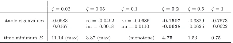
two stable eigenvalues are -0.1507 and -0.0638, respectively. Thus, the speed of convergence of
any variable at any point in time is a weighted average of the two stable eigenvalues. Over time,
the weight of the smaller eigenvalue (-0.1507) declines, hence the larger eigenvalue (-0.0638)
describes the asymptotic speed of adjustment.17 The flexibility provided by the additional
eigenvalue allows the model to match some features of the data, in particular with respect to
the current account.
Impact effects
The impact and long-run effects of an unanticipated permanent 100 percent increase in the oil
price are reported in bold in the second column of table 3. Starting off from the base equilibrium,
the 100 percent rise in the oil price leads producers to reduce oil input instantaneously around
41 percent. The marginal product of labor is reduced, and given the real wage, labor demand
falls. The impact reaction of firms is thus quite the same, regardless of the specific form of
preferences.
However, the reaction of households differs dramatically. The presence of a reference
con-sumption stock dampens the utility associated with a change in initial concon-sumption relative to
the reference stock and makes agents more reluctant to change their consumption pattern. This
is the “status effect” described by Alvarez-Cuadrado, Monteiro, and Turnovsky (2004). The
negative wealth effect of the oil price shock impacts on consumption expenditures (E) with a
0.98 percent reduction only. The marginal rate of substitution between consumption and leisure
increases, and at the going real wage, agents increase their labor supply, however at a smaller
amount compared to the conventional preferences case, because the marginal rate of substitution
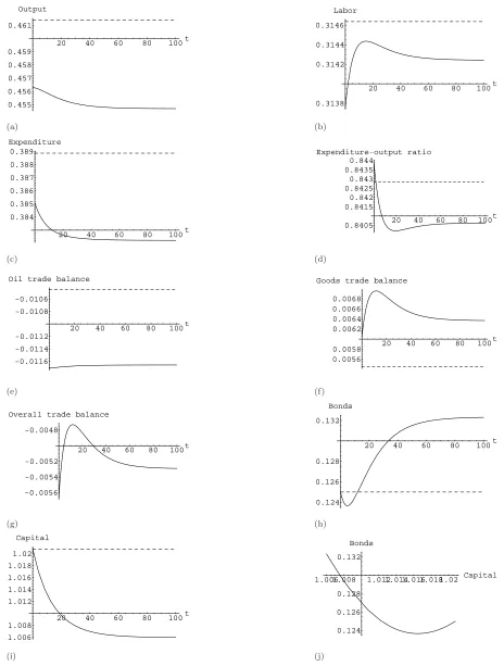
20 40 60 80 100t 0.455 0.456 0.457 0.458 0.459 0.461 Output (a)
20 40 60 80 100t
0.3138 0.3142 0.3144 0.3146 Labor (b)
20 40 60 80 100t
0.384 0.385 0.386 0.387 0.388 0.389 Expenditure (c)
20 40 60 80 100t 0.8405 0.8415 0.842 0.8425 0.843 0.8435 0.844
Expenditure-output ratio
(d)
20 40 60 80 100t
-0.0116 -0.0114 -0.0112 -0.0108 -0.0106
Oil trade balance
(e)
20 40 60 80 100t
0.0056 0.0058 0.0062 0.0064 0.0066 0.0068
Goods trade balance
(f)
20 40 60 80 100t
-0.0056 -0.0054 -0.0052 -0.0048
Overall trade balance
(g)
20 40 60 80 100t
0.124 0.126 0.128 0.132 Bonds (h)
20 40 60 80 100t
1.006 1.008 1.012 1.014 1.016 1.018 1.02 Capital (i)
1.0061.008 1.0121.0141.0161.0181.02 Capital
[image:23.595.65.529.92.705.2]0.124 0.126 0.128 0.132 Bonds (j)
changes less, due to the “status effect”. On the labor market, the reduction in labor demand
overweighs the increase in labor supply, the real wage drops, and hence employment falls by 0.28
percent. Given the capital stock, output drops by 1.11 percent. Compared to the conventional
case, output drops by a larger amount. The reason is the reduction in labor and oil input,
whereas in the conventional case labor input increases, dampening thus output reduction. In
figures 1(a), (b) and (c) the drops in output, labor, and consumption expenditures are
illus-trated by the difference between the dashed and solid lines.18 Because of the “status effect”,
the expenditure-output ratio increases, as figure 1(d) illustrates.
Instantaneous welfare of the representative agent falls now by 3.23 percent, meaning that
the agent is indifferent between the shock and a 3.23 percent reduction in his instantaneous
consumption levels of the traded good and oil.
Oil input and oil consumption both fall, but valued at the higher oil price, the value of
oil imports increases, hence the (negative) oil trade balance (OT B) deteriorates by roughly 12
percent. This is shown in figure 1(e).19
Investment expenditures are reduced because of the drop in the marginal productivity of
capital. The reductions in consumption of the domestically produced good and investment
expenditure are larger than the output drop, hence the (positive) goods trade balance (GT B)
improves by 10.95 percent, see also figure 1(f). However, the improvement is much smaller as
in the conventional preferences case (where it was 61.55 percent), because the “status effect”
dampens the consumption response to the oil price shock and increases the output reaction. The
improvement in the goods trade balance is not sufficient to outweigh the deteriorated oil balance,
and the (negative) overall trade balance deteriorates by about 13.30 percent, as illustrated in
1(g)20 The increased overall trade deficit starts a decumulation of net foreign assets, shown in
figure 1(h) by an initially downward-sloping time path of bonds.
Dynamic adjustments
The cut in investment expenditure initiates a decumulation of the capital stock. The dynamic
evolution of the capital stock is monotonic and illustrated in figure 1(i). The half-time of the
capital stock adjustment is roughly 9.7 years. Compared to the conventional case, this means
that the adjustment in the capital stock is fastened. Thus, the introduction of a reference
consumption stock counter-intuitively speeds up the dynamics.21
18The dashed lines refer to the base equilibrium.
19We have not drawn the time paths for C
i,Mi, and Zi. Their time paths are similar to that of expenditure
Ei and outputYi. This is becauseCi,MiandEimove proportionally according to equations (3a) and (3b), and
Ziis proportional toYi, as equation (3d) states.
20In the figure, the dashed line, illustrating the base equilibrium, and the horizontal axis coincide.
As time proceeds, because of reduced consumption expenditures the reference stock
grad-ually declines. This in turn makes agents less reluctant to further reduce their consumption
expenditures over time, as can be seen in figure 1(c). At the same time, together with falling
expenditures agents reduce their leisure and thus increase their labor supply, and in the earlier
stage of the dynamic transition firms are willing to hire more labor. Hence, employment
in-creases over roughly 15 years following the shock. However, the gradual, but ongoing reduction
of the capital stock reduces marginal productivity of labor, and firms become more and more
reluctant to hire additional labor. In fact, beyond 15 years, labor employed begins to fall slightly
towards its steady-state level. A can be seen from table 3, the difference between the impact
and steady-state change of oil input is extremely small (0.206 percentage points), implying that
almost all of the oil input adjustment happens instantaneously after the shock hits the economy.
The falling capital stock and reduced labor (which is always below the base level) lead to an
ongoing output reduction. As figure 1(a) reveals, in the very early stage of adjustment output
falls at an increasing amount, as capital decumulation is highest there, whereas after roughly 9.5
years output decline slows down. The evolution of the expenditure-output ratio is illustrated in
figure 1(d). After the initial increase it starts to fall, quickly achieving levels below the base line
and partially recovering in the latter stage of the dynamic adjustment.
The most interesting part of the dynamics is the evolution of the trade balance and its
components, and the time path for traded bonds. First, the oil trade balance slightly improves
during transition, as firms and households further cut back their oil usages. However, the
improvement of the oil balance is small. This can also be seen in table 3, which reveals that the
impact and steady-state changes of the oil trade balance differ only by roughly 0.5 percentage
points. Second, output, consumption and investment dynamics lead to an improving goods
trade balance in the first 11.47 years of transition. After that time, the ongoing reduction in
output overweighs the cut backs in investment expenditures (because more than half of the
capital stock’s adjustment is already done) and consumption expenditures on the domestically
produced good, and the goods trade balance deteriorates. Third, putting the time paths of the
oil balance and the goods trade balance (figures 1(e),(f)) together gives the evolution of the
overall trade balance. Improvements of the goods trade balance and the oil balance raise the
trade balance. Since almost all adjustment of the oil trade balance happens on impact, the
dynamics of the overall trade balance are almost entirely governed by the goods trade balance,
hence the phase of trade balance improvements ends slightly after that of the goods trade balance
(i. e. after roughly 11.76 years). From thereon, the trade balance deteriorates towards its new
Taking interest income on traded bonds into account, the accumulation of bonds (and hence
the current account) evolves as depicted in figure 1(h). Traded bonds are decumulated, but this
decumulation slows down, and after 4.75 years the current account reverts into a surplus. From
thereon, bonds are accumulated, and at steady-state the economy has improved its net foreign
asset position. The reason for this quite early switch in the current account stems from the fact
that the overall trade balance returns quickly (after roughly 4.25 years) to its pre-shock level.
Because during this time the stock of bonds declined, interest income has fallen, and hence the
current account turns into surplus a little bit later.
The evolution of traded bonds and hence of the current account shows the J-curve
prop-erty. After the increase in the oil price (the deterioration in the country’s terms of trade), the
current account worsens instead of improving, and it takes some time until the current account
switches back to a “normal” reaction upon a deterioration in the terms of trade. By comparing
the benchmark economy with time non-separable preferences with the conventional one, it is
clear that the model’s J-curve phenomenon is due to the presence of consumption habits. The
emergence of a J-curve when habit formation is present is described in detail by Cardi (2007),
although his model is different in several aspects.22 Since the oil trade balance remains almost
constant, it is the reduced change in consumption expenditures on the domestically produced
good, due to the “status effect”, which causes the J-curve. This J-curve effect can also be seen
in the state-space representation ofK andB in figure 1(j). In the conventional preferences case,
the trajectory would be a negatively sloped line.
Steady state effects
As the second column of table 3 reveals, in the long run output and the capital stock fall by 1.45
percent (w. r. t. the base equilibrium), and labor is reduced by 0.13 percent. Oil input usage
is cut back by 41.40 percent, and consumers reduce their expenditures by 1.71 percent. The
(positive) goods trade balance improves by 16.79 percent, whereas the oil balance deteriorates
by 11.57 percent, resulting in an overall deterioration of the (negative) trade balance by 5.88
percent. Accordingly, the steady-state net foreign asset position (positive) has to rise by 5.88
percent. The long-run oil share (OT B/Y) increases by 13.21 percent and is still fairly low at
0.02564.
Perhaps most important from the point of view of the representative agent is the change in
his intertemporal welfareW. The 100 percent oil price hike lowers the agent’s overall welfare by
22In Cardi’s model, (i) agents are “inward-looking”, (ii) labor is fixed, (iii) they are no imported inputs, and
2.35 percent in the sense that he is indifferent between the shock and a 2.35 percent reduction
in his permanent consumption levels of the traded good and oil.
Compared to the case of conventional preferences, the model with a reference consumption
stock matches data much better, predicting that after an oil price shock, the economy suffers a
slump, as output drops, employment falls, and the current account worsens. A large amount of
the total steady-state output change occurs right on impact, a feature which is stressed by many
empirical studies, see, e. g., Jim´enez-Rodr´ıguez and S´anchez (2004), Blanchard and Gal´ı (2007),
and Kilian (2007). The dynamic evolution of the current account confirms the early findings
of Agmon and Laffer (1978), and more recently of Rebucci and Spatafora (2006) and Kilian,
Rebucci, and Spatafora (2007). Moreover, compared to the conventional model, the long-run
change in the overall trade balance is strongly reduced. With respect to the output loss, the
model fits actual findings that this loss is quite low. The long-run loss (-1.45 percent) is in
accordance of what, e. g., Jim´enez-Rodr´ıguez and S´anchez (2004) the OECD (2004), Nordhaus
(2007), Blanchard and Gal´ı (2007) and Schmidt and Zimmermann (2007) found.
6
Sensitivity analysis
Having discussed the dynamics and the steady-state changes, we now perform some sensitivity
analysis with respect to the weight γ of the reference consumption stock in preferences, the
speed of adjustment ζ of the reference consumption stock, and the oil share in output.
6.1 Weight of habits in preferences
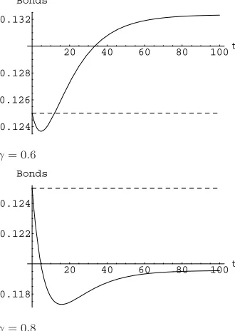
Starting from the benchmark calibration, we will vary the weight γ from zero to 0.8, as recent
empirical evidence suggests values of γ up to 0.9. We already discussed in detail the case of
γ = 0, when the evolution of the reference stock becomes irrelevant. The results of the sensitivity
analysis are summarized in columns one to four of table 3. Asγ increases, the smaller stable root
increases (becomes less negative), whereas the larger stable root falls (becomes more negative).
Hence, the asymptotic speed of convergence increases withγ. The half-time of the capital stock
falls with an increasing γ, whereas the duration of the current account deficit rises.
In the short run, an increasingγraises the initial output loss, increases the reductions in labor
and oil input, and lowers agents’ expenditure cuts and therefore the change in the goods trade
balance. As agents are increasingly reluctant to cut their consumption expenditures, they are
increasingly unwilling to increase their labor supply, resulting in increasingly lower employment.
The cut in oil input is almost not affected, as preferences impinge on the production side of
(negative) overall trade balance becomes increasingly negative with rising γ. The instantaneous
welfare loss rises with γ, too.23 In the long run, the higher γ, the lower the steady-state
20 40 60 80 100t
0.125 0.135 0.14 0.145 0.15 0.155 0.16
Bonds
γ= 0
20 40 60 80 100t
0.124 0.126 0.128 0.132
Bonds
γ= 0.6
20 40 60 80 100t
0.123 0.124 0.125 0.126
Bonds
γ= 0.7
20 40 60 80 100t
0.118 0.122 0.124
Bonds
[image:28.595.356.521.110.342.2]γ= 0.8
Figure 2: Time paths of bonds for different weights of habits
reductions in output and the capital stock, and the smaller the reduction in labor. Agents’
long-run expenditure change increases with γ. The improvement of the (positive) goods trade
balance becomes larger. Because the long-run oil balance is insensitive to γ, the (negative)
steady-state trade balance deteriorates less as γ increases, and forγ = 0.8 it improves. These
changes are mirrored in the net foreign asset position. The long-run welfare loss rises with γ.
The reason for this sensitivity with respect to γ is that in the short run an increase in the
weight of habits makes agents more reluctant to reduce their expenditures and to supply more
labor, increasing thus the output loss, the trade balance deficit and hence the current account
deficit, leading in turn to a longer period of bonds decumulation and to more pronounced
changes in the the net foreign asset position. Because agents are forward-looking, an increasing
reluctance to reduce consumption expenditures on impact requires a larger long-run expenditure
cut to maintain intertemporal solvency. On the other hand, larger long-run consumption cuts
increase agents’ willingness to supply labor, thus reducing the steady-state drops in employment,
output, and the capital stock.
The case ofγ = 0.8 is of particular interest, as some empirical work suggests this high value
for a lot of countries. In that case, the economy ends off with a lower stock of traded bonds. For