Munich Personal RePEc Archive
Estimation and inference in unstable
nonlinear least squares models
Boldea, Otilia and Hall, Alastair R.
University of Tilburg, University of Manchester
20 May 2010
Online at
https://mpra.ub.uni-muenchen.de/23150/
Estimation and Inference in Unstable Nonlinear
Least Squares Models
∗
Otilia Boldea
†and Alastair R. Hall
‡May 20, 2010
∗We are grateful to Philippe Berthet, Mehmet Caner, Manfred Deistler, John Einmahl,
At-sushi Inoue, Denise Osborn, James Stock and Qiwei Yao for their comments, as well as for the comments of participants at the presentation of this paper at the Conference on Breaks and Persistence in Econometrics, London, UK, December 2006, Inference and Tests in Economet-rics, Marseille, France, April 2008,European Meetings of the Econometric Society, Milan, Italy, August 2008,NBER-NSF Time Series Conference, Aarhus, Denmark, September 2008,Fed St. Louis Applied Econometrics and Forecasting in Macroeconomics Workshop, St. Louis, October 2008, and at the seminars in Tilburg University, University of Manchester, University of Exeter, University of Cambridge, University of Southampton, Tinbergen Institute, UC Davis and Insti-tute for Advanced Studies, Vienna. The second author acknowledges the support of ESRC grant RES-062-23-1351.
†Corresponding author. Tilburg University, Dept. of Econometrics and Operations Research,
Warandelaan 2, 5000 LE Tilburg, Netherlands, Email: [email protected]
Abstract
In this paper, we extend Bai and Perron’s (1998, Econometrica, pp. 47-78) method for detecting multiple breaks to nonlinear models. To that end, we consider a nonlinear model that can be estimated via nonlinear least squares (NLS) and features a limited number of parameter shifts occur-ring at unknown dates. In our framework, the break-dates are estimated simultaneously with the parameters via minimization of the residual sum of squares. Using new uniform convergence results for partial sums, we derive the asymptotic distributions of both break-point and parameter estimates and propose several instability tests. We provide simulations that indicate good finite sample properties of our procedure. Additionally, we use our methods to test for misspecification of smooth-transition models in the con-text of an asymmetric US federal funds rate reaction function and conclude that there is strong evidence of sudden change as well as smooth behavior.
JEL classification: C12, C13, C22
1
Introduction
As pointed out by Lucas (1976), policy shifts and time-varying market
condi-tions induce behavioral changes in the decisions of economic agents. Hence, over
longer time spans, a stable model might not be the appropriate tool to capture the
features of economic decisions. A popular way to capture instability in
macroe-conometric models is to impose sudden parameter shifts at unknown dates, known
as break-points.
Both the econometric and statistical literature on break-point problems is
ex-tensive1, and its main focus is on testing for breaks rather than estimation. For
example, early work by Quandt (1960) suggests using a supremum (sup) type test for inference on a single unknown break-point. Whether in linear or nonlinear
set-tings, most subsequent work - seeinter aliaAnderson and Mizon (1983), Andrews and Fair (1988), Ghysels and Hall (1990), Andrews (1993), Sowell (1996), Hall
and Sen (1999) and Andrews (2003) - proposes tests that are designed against the
alternative of a one-time parameter variation or of more general model
misspeci-fication. For parametric settings, Bai and Perron (1998) is among the few papers
that propose tests for identifying multiple breaks. Their tests are designed for
linear models estimated via ordinary least-squares (OLS). While these tests are
useful, the linear framework might be considered a limitation. Subsequent papers
such as Kokoszka and Leipus (2000), Lavielle and Moulines (2000) and Andreou
and Ghysels (2002) propose tests for parameter instability in nonlinear models,
but the nonlinearities considered are confined to special cases such as general
autoregressive conditional heteroskedasticity (GARCH) models. The framework
considered in this paper is more general, imposing only mild restrictions on the
nonlinear regression function.
1For statistical literature surveys, see Zacks (1983), Krishnaiah and Miao (1988),
In practice, researchers often argue that it can be difficult to discriminate
between misspecification due to parameter instability or neglected nonlinearity.
It is therefore desirable to develop a framework that allows both features. While
tests such as the ones developed in Eitrheim and Ter¨asvirta (1996) can detect
instability in some classes of nonlinear models, they are not particularly designed
against an alternative with breaks nor offer an estimation framework that can
allow for both smooth and sudden change. One of the aims of this paper is to
provide change-point tests in the spirit of Bai and Perron’s (1998) tests, but with
a maintained nonlinearity assumption. These tests are valid for a large class of
parametric nonlinear models, includinginter aliasmooth transition models, neural networks, partially linear, bilinear and (nonlinear) GARCH models.
Compared to inference procedures, the issue of consistently estimating one or
multiple change-points - when their location is unknown - has received
consider-ably less attention in the literature. Within linear parametric models, there are
a few methods that yield consistent estimates of the break-points, e.g. maximum
likelihood - Quandt (1958), least-squares - Bai (1994), least absolute deviation
- Bai (1995), information criteria - Yao (1988), Davis, Lee, and Rodriguez-Yam
(2006). In Bai and Perron’s (1998) paper, the break points are estimated
simulta-neously with the regression parameters via least-squares methods. Bai and Perron
(1998) establish consistency and derive the convergence rate of the resulting break
point fractions under fairly general assumptions. They also propose a sequential
procedure for selecting the number of break points in the sample based on various
tests for parameter constancy. This procedure is extended to models with
cross-regime restrictions by Perron and Qu (2006), and to multivariate frameworks by
Qu and Perron (2007). Hall, Han, and Boldea (2009) further extend Bai and
Perron’s framework to linear models with endogenous regressors. A slightly
differ-ent approach is proposed by Davis, Lee, and Rodriguez-Yam (2006); they suggest
via minimization of the minimum description length (MDL) criterion of Rissanen
(1989).
While useful, all the analyses above are restricted to linear models with breaks,
which are often unsuitable for the asymmetries macroeconomic behavior displays.
To capture these asymmetries, nonlinear models are becoming increasingly
pop-ular, and there is a need to develop tests and inference procedures for multiple
parameter changes in this setting.
In this paper we consider a univariate nonlinear model that can be estimated
via NLS - or under stronger assumptions, equivalent methods such as
quasi-maximum likelihood - and exhibits multiple unknown breaks. Allowing for
non-stationary but piece-wise ergodic regressors and errors, we show that a
minimiza-tion of the sum of squared residuals over all possible break dates and parameters
yields consistent estimates of both the unknown break fractions and parameters.
We further prove T-rate convergence of break fraction estimates, a key result
because it implies that inference on parameters can be conducted as if the
break-points were known a priori. To obtain this result, we arrive at one of the main contributions of our paper: a new uniform central limit result for piece-wise ergodic
and mixing processess, which may be useful in other contexts.
Based on the above, we provide various structural stability tests - in the
pres-ence or abspres-ence of autocorrelation - that naturally generalize those proposed by
Bai and Perron (1998). We consider global tests of no breaks against two types
of alternative, one in which the number of breaks is fixed and another in which
the number of breaks is only restricted to be less than some ceiling, along with
sequential tests for an additional break. These tests can be used to develop a
sequential method for finding the number and locations of breaks, as suggested
by Bai and Perron (1998) in linear settings. Moreover, the sequential Wald test
we propose - similar to Hall, Han, and Boldea (2009) - allows for breaks in the
number of breaks to settings where autocorrelation is present.
For forecasting purposes, it is still of interest to know with certain confidence
when the last break occurred. As Bai (1994, 1995, 1997) shows, change-point
distributions in linear models can be derived in two cases: when the magnitude of
parameter shifts is constant and when it shrinks to zero at a certain rate. Because
in the first case, the confidence intervals depend on the distribution of the data, the
device of shrinking shifts is used to ensure that shifts disappear at a slow enough
rate so that pivotal statistics can still be obtained. In practice, this framework
can be viewed as one of moderate shifts, according to Bai and Perron (1998). A
local analysis of small shifts is presented in Elliott and M¨uller (2007) for linear
models, but providing a similar framework here is beyond the scope of our paper.
We consider each of the two cases above in turn. For the first case, we
pro-vide an asymptotic approximation to the exact change-point distribution, but this
approximation is - as for linear cases its exact counterpart - dependent on the
distribution of the data. For the second case, we obtain a similar asymptotic
dis-tribution as in Bai (1997). We validate the usefulness of our estimators, tests and
confidence intervals via simulations.
Next, we illustrate our methodology in the context of the US interest rate
reaction function. Using a similar setup to Kesriyeli, Osborn, and Sensier (2006),
we test a STR model with one-transition and find evidence of both smooth and
sudden change.
The paper is organized as follows: Section 2 describes our model. Section
3 reveals the assumptions needed for our estimation method. We outline the
consistency and limiting distributions results in Section 4. Section 5 rederives
-in a nonl-inear context - two classes of stability tests. Section 6 shows good f-inite
properties of our break-point estimators, tests and number of break-points. Section
7 applies the methods proposed in this paper to an interest rate reaction function
the detailed proofs can be found in a Supplemental Appendix that is available
from the authors upon request.
2
Model
In this section, we introduce a univariate nonlinear model withmunknown
change-points:
yt=f(xt, θ0i+1) +ut t∈Ii0 = [Ti0+ 1, Ti0+1] i= 0,1, . . . m (1)
where T0
0 = 0 andTm0+1 = T by convention. Here yt is the dependent variable,
xt(q×1) are the regressors, θ0
i+1 (p×1) are parameters that change at dates Ti0, f : Rq ×Θ → R is a known measurable function on R for each θ ∈ Θ, and T is
the sample size. To begin, we consider m to be a known finite positive integer,
but we allow for the break dates to be unknown to the researcher; we consider the
question of how to estimatem in Section 6. For simplicity, letft(θ) =f(xt, θ) and
denote by ¯Tm ≡ (T
0 = 1, T1, . . . , Tm, Tm+1 = T) any m-partition of the interval
[1, T]. To further simplify the notation, we will stack column vectors such as θ0
i+1
and θi+1 into two corresponding (m + 1)p× 1 vectors, θc0 and θc. For a given
sample partition and given parameter values θc, denote by S
T( ¯Tm, θc) the sum of
squares.2
One of our main goals is to provide a method for estimating the unknown
pa-rameters and change points. As in Bai and Perron (1998), the estimation method
we propose is based on the least-squares principle3 and follows in two steps. First,
2We use superscriptcto distinguish between (m+ 1)p×1 parameter vectors and the p×1
parameter vectors at whichft(·) is evaluated.
3Note that an extension to more general settings such as generalized method of moments
we obtain the sub-sample NLS estimators for each partition:
ˆ
θcT( ¯Tm) = argmin
θc( ¯Tm)
ST( ¯Tm, θc( ¯Tm) ) (2)
Second, we search over all possible partitions to obtain the break-point estimates.
The estimates ˆT = (1,Tˆ1, . . . ,Tm, Tˆ ) for change-points and ˆθcT = (ˆθ1, . . . ,θmˆ +1) for
parameters are obtained as follows:
ˆ
T = argmin
¯
Tm
ST ( ¯Tm,θˆcT( ¯Tm) ) and ˆθTc = ˆθcT ( ˆT) (3)
The above is an NLS estimation with an appropriate modification to allow for
mul-tiple break-points, and can be legitimately performed provided thatE[utft(θ0
i+1)] =
0 for each t=T0
i + 1, . . . , Ti0+1 (i= 0,1, . . . m).
3
Assumptions
To derive the statistical properties of our estimators, we establish a framework
that combines elements of asymptotic theory in stable nonlinear models and
un-stable linear models. As pointed out by Hansen (2000), the marginal distributions
of regressors and/or errors may change, possibly at different locations in the
sam-ple than the population parameters of the equation of interest. Our framework
is designed to achieve as much generality as possible with respect to changes in
marginal distributions,4 as well as with respect to other non-stationarities induced
by lagged dependent variables that may enter the model concomitantly with
pa-rameter breaks. In dealing with nonlinear asymptotics, we impose usual
smooth-ness and boundedsmooth-ness assumptions. To deal with instability, we assume uniform
4Allowing for these types of changes is important in many settings. For example, when
convergence of certain quantities, jointly in parameters and a partial sum index.
Assumption 1. Let vt= (x′
t, ut)′. Then:
(i) {vt} is a piece-wise geometrically ergodic process, i.e. for some finite m∗ >0
and each sub-sample [T∗
j−1+ 1, Tj∗], where Tj∗ = [T λ∗j], j = 0, . . . , m∗+ 1, λ∗0 = 0<
λ∗
1 < . . . < λ∗m∗ < λ∗m∗+1 = 1, there exists a unique stationary distribution Qj such
that:
sup
A |
P(A|B)−Qj(A)| ≤gj(B)ρt
with 0 < ρ < 1, A ∈ FT
∗
j
T∗
j−1+t, B ∈ F
T∗
j−1
−∞ , Fkl is the σ-algebra generated by
(vk, . . . , vl), and gj(·) is a positive uniformly integrable function. If {xt} does not contain lagged dependent variables, then the assumption above holds with {vt}
augmented by yt.
(ii) {vt} is a β-mixing process with exponential decay, i.e. there existsN >0 such that for B ∈ Fa
−∞,
βt= sup
a
β(F−∞a ,Fa∞+t)≤Nρt
β(Fa
−∞,Fa∞+t) = sup A∈F∞
a+t
E|P(A|B)−P(A)|
(iii) E[utft(θ)] = 0 for each θ ∈Θ.
Assumption 2. The function ft(·)is a known measurable function, twice contin-uously differentiable in θ for each t.
Assumption 3. Let Ft(θ) =∂ft(θ)/∂θ, p×1vector and ft(2)(θ), ap×pmatrix of
second derivatives, i.e. ft(2)(θ) = ∂2ft(θ)/(∂θ∂θ′), with (i, j)th element f(2)
t,i,j. Also
denote by k · k the Euclidean norm. Then (i) the common parameter spaceΘ is a compact subset of Rp; for some s >2, we have: (ii) sup
t,θE|utft(θ)|2s <∞; (iii)
supt,θEkutFt(θ)k2s <∞; (iv) For i, j = 1, . . . p, supt,θEkutf
(2)
Assumption 4. (i) S(θc) = plim T−1ST(θc) has a unique global minimum at
θc
0; (ii) Let Ai,T(θi0) = Var T−1/2
P
t∈I0
i−1 utFt(θ
0
i), for i = 1, . . . , m+ 1, and AT(θ, r) = Var T−1/2 P[T r]
t=1 utFt(θ). Then Ai,T(θi0) p
→ Ai(θ0
i), and AT(θ, r) p → A(θ, r), where the two limits are finite positive definite matrices not depending on T, and the latter convergence holds uniformly in θ×r ∈ Θ×[0,1]. (iii) Let
Di,T(θ0
i) = T−1
P
t∈I0
i−1Ft(θ
0
i)Ft(θi0)′ and DT(θ, r) = T−1
P[T r]
t=1 Ft(θ)Ft(θ)′. Then
Di,T(θ0
i) p
→Di(θ0
i) andDT(θ, r) p
→D(θ, r), where the two limits are finite positive definite matrices not depending on T, and the latter convergence holds uniformly in θ×r∈Θ×[0,1]; (iv) E[ft(θ0
i)]6=E[ft(θ0i+1)], for each i= 1,2, . . . , m.
Assumption 5. Ti0 = [T λ0i], where 0< λ01 < . . . < λ0m <1.
Assumption 1(i) can be interpreted as asymptotic stationarity of {vt} within
regimes, and it allows for breaks in the marginal distribution of regressors and
errors.5 Additionally, it allows for ‘temporary’ nonstationary behavior, which
is especially useful in the presence of lagged dependent variables, in which case
(1) may induce recurring changes in their marginal distribution. In this case,
Assumption 1(i) ensures that even if the process yt starts in a certain regime at
a draw from the nonergodic distribution, it converges to the stable distribution of
that regime, so enough homogeneity in the process is preserved to ensure that a
uniform central limit theorem still holds in that particular regime.6
Assumption 1(ii) ensures that the dependence within and among sub-samples
dies out at the same rate as the ergodicity rate. Ifm∗ = 0, {vt} admits a Markov
5Note thatm∗ as well asλ∗
j are taken as given and are not objects of inference here, unless all breaks in{vt}either are aligned or coincide with the breaks the parameters of (1), depending on whether {xt} contains lagged dependent variables or not. When the breaks in {vt} are neither aligned nor coincide with the parameter breaks, knowledge of λ∗
j is irrelevant as far as asymptotic distribution results are concerned, but may be of course crucial for both getting consistent estimates of certain asymptotic variances, as well as obtaining the null distribution of stability tests - see Hansen (2000) and Section 5.
6In the absence of lagged dependent variables, we need piece-wise ergodicity off
chain representation and is geometrically ergodic as in Assumption 1(i), then {vt}
is β-mixing with exponential decay, subject to an absolute continuity condition
on the starting values - see e.g. Rosenblatt (1971), Mokkadem (1985) - and this
connection is often exploited in nonlinear GARCH models - see e.g. Carrasco and
Chen (2002). If {vt} is a Markov chain, but m∗ > 0, then piece-wise geometric
ergodicity only implies that theβ-mixing coefficients on those sub-samples (thus,
for restrictedσ-algebras) are exponentially decaying, and we could allow for slower
decay across sub-samples. For coherence purposes, we stick to Assumption 1.
Assumption 1(iii) also ensures that the model can be estimated via NLS, since
the errors are uncorrelated with the regression function. Assumption 2 and 3
are typical smoothness and boundedness assumptions encountered in nonlinear
models.
Assumption 4 (i) is the usual NLS identification assumption. Assumptions 4
(ii) and (iii) allow substantial heterogeneity in the second moments of regressors
and errors. Assumption 4 (iv) ensures that the parameter shifts across regimes can
be identified. Assumption 5 is a typical assumption for unstable models, allowing
the break-fractions to be fixed and hence the break-points to be asymptotically
distinct.
4
Asymptotic Behavior of Estimates
4.1
Consistency of Break-Fraction Estimates
In Section 2, we described a least-squares based method similar to its linear
coun-terpart in Bai and Perron (1998). To elucidate the connection between linear
and nonlinear settings, we will provide a heuristic discussion first. As Gallant
(1987) shows, NLS estimators have the same form as OLS estimators (in stable
models) up to a first-order approximation. To see that, denote by X the T ×q
F =∂f(X, θ0)/∂ θ, where θ0 is the true parameter value. The similarity between OLS and NLS can be seen from the equation below:
OLS= (X′X)−1X′y; NLS = (F′F)−1F′y+o
p(T−1/2) (4)
Given this similarity, extending Bai and Perron’s (1998) methodology to
non-linear settings may seem straightforward. However, consistency of parameters
estimates, and related to this, the Taylor expansion needed to obtain a similar
for-mula as in (4) for unstable NLS estimates cannot be legitimately obtained prior
to deriving the consistency and convergence rate of break-fraction estimates. For
the latter we require different proof strategies, but the results are similar to Bai
and Perron (1998) and are summarized in Theorems 1 and 2.
Theorem 1. For each i = 1, . . . , m, let λiˆ be the smallest number such that
ˆ
Ti = [Tˆλi]. Then, under Assumptions 1-5, λˆi p − →λ0
i.
For intuition and because they are informative for Assumption 1, we outline
the main steps of the proof here, the details being relegated to the Appendix.
Define ˆut=yt−ft(ˆθk+1), fort ∈Iˆk and dt = ˆut−ut=ft(θj0+1)−ft(ˆθk+1), for
t∈I0
j ∩ Ikˆ, with Ij0 = [Tj0+ 1, Tj0+1] and ˆIk = [ ˆTk+ 1,Tkˆ+1] andk, j = 0,1, . . . , m.
Also, denote ψt(θ) = utft(θ), a mean zero process governed by Assumption 1.
Then:
T−1
T
X
t=1
utdt =T−1 m
X
i=0
X
I0
i
ψt(θ0i)−T−1 m
X
i=0
X
ˆ
Ii
ψt(ˆθi) =I+II.
The proof of consistency rests on showing thatI+II isop(1). WhileI =op(1)
by a simple law of large numbers, the analysis of II is more complicated as this
term contains not only sums with random endpoints but summands that depend
on the parameter estimators, which in turn depend on the random endpoints. In
Lemma 1. Under Assumptions 1-2 and 3(i)-(ii), QT(θ, r) =T−1/2P[T r]
t=1 ψt(θ) =
Op(1) uniformly in θ×r ∈Θ×[0,1].
Lemma 1 was shown by Caner (2007) under the assumption that {vt}, and
hence {ψt(θ)}, is a strictly stationary process. In this paper, we relax strict
sta-tionarity over the whole sample to piece-wise ergodicity, in which case even though
QT(θ, r) does not have a unique limit for all r, the uniform boundedness result
in Lemma 1 holds. Our result applies to a large class of nonlinear models
in-cluding smooth transition autoregressive models, other nonlinear autoregressive
models, neural networks, partially linear models, nonlinear GARCH models,
with-out further restrictions on the functional form of ft(θ) besides those imposed in
Assumption 2.
With Lemma 1 in mind and using the definition of the sum of squared residuals,
one can show that:
T−1 T
X
t=1
d2t + 2T−1 T
X
t=1
dtut≤0 (5)
Consistency follows from the following lemma:
Lemma 2. Let Assumption 1-5 hold. ThenT−1PT
t=1utdt =op(1); (ii) If λjˆ
p
9λ0
j
for some j, then lim sup P hT−1PT
t=1d2t > C
i
> ǫ, for some C >0, ǫ > 0.
Given part (i) of Lemma 2 and inequality (5), it follows that T−1PT
t=1d2t = op(1). The latter is in contradiction with part (ii) of Lemma 2, establishing
con-sistency of break-fraction estimates.
4.2
Rates of Convergence
A necessary next step involves determining the convergence rates of the
break-fraction estimates. The results are summarized below:
Theorem 2. Under Assumptions 1-5, for everyη >0, there exists a finite C >0
such that for all large T, P(|T(ˆλk−λ0
Theorem 2 is useful since the consistency of ˆθTc can be established provided that
the difference between the estimated and the true objective function is no more
than op(1). This is the case here because Theorem 2 implies that the difference
involves a bounded number ofop(1) terms. Given theT-rate convergence of
break-fraction estimates, the limiting distributions of parameter estimates follow from
standard NLS asymptotics:
Theorem 3. Under Assumptions 1-5, θiˆ and θjˆ are asymptotically independent and T1/2(ˆθi − θ0
i) d
→ N (0,Φi(θ0i)), where Φi(θi0) = [Di(θi0)]−1Ai(θi0)[Di(θ0i)]−1
for i, j = 1, . . . , m+ 1, i6=j.
Theorems 1-3 allow us to estimate the covariance matrices Φi(θ0i) by replacing Di(θ0
i) with ˆDi(ˆθi) =T−1
PTˆi
t= ˆTi−1+1Ft(ˆθi)Ft(ˆθi)
′ and Ai(θ0
i) with a
heteroskedas-ticity and autocorrelation (HAC) robust covariance matrix estimator, ˆAi(ˆθi). If
more structure is placed on the data, then the form of Φi(θi0) simplifies and thus
so does the form of its consistent estimator. The following example considers an
important special case.
Assumption 6. (i) Assumption 1 holds with m = m∗, T∗
i = Ti, i = 1, . . . , m if {vt}does not contain any lagged dependent variables. Ifvtcontains lags ofyt, then Assumption 1 holds with m∗ =m with T∗
i =Ti, i= 1, . . . , m but for vt∗ ={yt, x∗t}
instead of{vt}, with x∗
t being all regressors besides the lagged dependent variables; E[ut|xt] = 0 and E[utus|xkxl] = 0 for all t 6= s and all k, l; (ii) The errors are homoskedastic within regimes: E[u2
t | xt] =
Pm+1
i=1 σi21{t ∈ Ii0} for all t; (iii)
Let DT,i(θ, r) = T−1PTi0−1+[T r]
t=T0
i−1+1 Ft(θ)Ft(θ)
′. Then DT,i(θ, r) →p rDi(θ), uniformly
in θ ×r ∈ Θ×[0, λ0
i −λ0i−1], where the latter is a positive definite matrix not depending on T, with Di(θ) not necessarily the same for all i; (iv) Let AT,i(θ, r) = Var T−1PTi0−1+[T r]
t=T0
i−1+1 ut(θ)Ft(θ). Then AT,i(θ, r)
p
→rAi(θ), uniformly in θ×r ∈
Θ×[0, λ0
i −λ0i−1], where the latter is a positive definite matrix not depending on
T, with Ai(θ) not necessarily the same for all i.7
Corollary to Theorem 3. Under Assumption 6, the covariance matrix in The-orem 3 simplifies to Φi(θ0i) = σi2[Di(θi0)]−1 and can be consistently estimated by
ˆ
σ2
i[ ˆDi(θi0)]−1, where σˆ2i = ( ˆTi−Tiˆ−1)−1 P ˆ
Ti
t= ˆTi−1+1uˆ
2
t, for i= 1, . . . , m+ 1.
Note that Assumption 6 allows for breaks in marginal distributions of
regres-sors, as well as breaks in the error variance that occur at the same time as the
true breaks in model (1).
4.3
Limiting Distribution of Break Dates
Similar work by Bai (1994, 1995, 1997) for linear models derives the non-standard
distributions of change-point estimates. Hall, Han, and Boldea (2010) extend
these results to models that can be estimated via two stage least squares. These
papers find the distribution of the break-point estimators in two cases, fixed and
shrinking magnitude of shifts. In the first case, in general, the distributions in
linear models depend on the underlying distribution of the regressors and errors.
The second case allows for magnitudes of shifts that shrink to zero as the sample
size increases. We consider both cases in turn.
4.3.1 Fixed Magnitude of Shifts
Consider the following data generation process, with one break8:
yt =
f(xt, θ0
1) +ut t = 1, . . . , k0
f(xt, θ0
2) +ut t =k0+ 1, . . . , T.
An implicit assumption so far was that the parameter shifts are constant:
Assumption 7. δ=θ0
2 −θ01, a fixed number.
8,9.
8The extension tombreaks is immediate because the impliedm+ 1 sub-samples are
Denote by ST(k, θ1, θ2) the sum of squared residuals evaluated at a potential
break-point 1 ≤ k ≤ T. Also, let ST(k) = minθ1,θ2ST(k, θ1, θ2). Then we can
write:
ˆ
k= argmin
1≤k≤T
argmin
θ1,θ2
V(k, θ1, θ2) (6)
where: V(k, θ1, θ2) = ST(k, θ1, θ2)−ST(k0, θ10, θ02). We obtain a large sample
ap-proximation to this finite distribution, given below:
Theorem 4. Under Assumptions 1-5 and 7, for m= 1,
h ˆ
k−k0
i
−argmax
v∈R
J∗(v)→p 0,
whereJ∗(v)is a double-sided stochastic process withJ∗(0) = 0, J∗(v) =J∗
1(v), v =
−1,−2, . . .; J∗(v) =J∗
2(v), v = 1,2, . . .; and
J1∗(v) =
k0
X
t=k0+v+1
ft(θ02)−ft(θ01)2
−2
k0
X
t=k0+v+1
ut
ft(θ20)−ft(θ01)
J2∗(v) =−
k0+v
X
t=k0+1
ft(θ20)−ft(θ10)2
−2
k0+v
X
t=k0+1
ut
ft(θ20)−ft(θ01)
The result above is comparable to linear models. If we assume that the errors
in (1) are independent of each other and of the regressors, J∗(v) becomes a
two-sides random walk with stochastic drifts. If we also impose strict stationarity of
{vt}in Assumption 1(i) with m∗ = 0, the limit is a two-sided Gaussian stochastic
process with negative drift, and it is the same as the limit for shrinking shifts (see
next section).
4.3.2 Shrinking Magnitude of Shifts
Instead of Assumption 7, consider Assumption 8, which imposes parameter shifts
Assumption 8. Fori= 1, . . . , m, =θi0+1,T−θ0i,T =δiwT, where δi are fixed p×1
vectors and {wT} is a scalar series such that wT → 0 and T1/2−γw2
T → ∞ as T → ∞, for some γ ∈
0,12
.
This assumption ensures that the asymptotic distributions of the change-point
estimates do not depend on the underlying distributions of {ut, ft(θ)}. Similar
assumptions areinter aliaT1/2−γwT → ∞, forγ ∈ 0,1 2
in Bai and Perron (1998)
and T1/2w
T/(logT)2 → ∞ in Qu and Perron (2007). Our assumption allows only
shifts of order T−1/4 or larger, but the simulation section discusses that, despite
this, the coverage probability for the confidence intervals is good. Note that under
shrinking magnitudes of shift, the asymptotic properties of parameter and
break-fraction estimates need to be re-derived (see Appendix), with the break-break-fraction
distribution presented below.
Theorem 5. Let φ = δ1′A2(θ01)δ1/[δ1′A1(θ01)δ1] and ξ = δ1′D2(θ01)δ1/[δ′1D1(θ10) δ1]. Under Assumptions 1-5, 6(iii)-(iv), and 8, for m= 1,
[δ′
1D1(θ10)δ1]2
δ′
1A1(θ10)δ1
wT2[ˆk−k0]⇒argmax
v
Z(v)
where Z(v) =J1(−v)−0.5|v|, v ≤0, Z(v) = √φJ2(v)−0.5ξ|v|, v >0, J1(v), J2(v) are two independent standard scalar Gaussian processes defined on[0,∞], and ‘⇒’ denotes weak convergence in Skorohod metric.
Details regarding this process can be found in Bai (1997). The density of
argmaxvZ(v) is characterized by Bai (1997) and he notes that it is not symmetric
if φ 6= 1 or ξ 6= 1. A confidence interval can be constructed as follows. Let
ˆ
ω1,i = (ˆθ2 −θˆ1)′Aiˆ(ˆθ1)(ˆθ2 − θˆ1), ˆω2,i = (ˆθ2 −θˆ1)′Diˆ (ˆθ1)(ˆθ2 −θˆ1), ˆDi(θ) = ( ˆTi −
ˆ
Ti−1)−1P ˆ
Ti
t= ˆTi−1+1 Ft(θ)Ft(θ)
′; ˆAi(θ) a HAC estimator of the long-run variance
Ai(θ), and ˆH = ˆω2
100(1−α)% confidence interval for ˆk is:
( ˆk − [c1/Hˆ]−1,kˆ + [c2/Hˆ] + 1 ) (7)
wherec1andc2are respectively the (α/2)thand (1−α/2)thquantiles for argmaxvZ(v)
which can be calculated using equations (B.2) and (B.3) in Bai (1997).
Theorem 5 can be extended to yield confidence intervals for the multiple break
model, because given Assumption 1, the sample segments are asymptotically
in-dependent, allowing for the analysis of the limiting distribution to be carried out
as in the one break case:
Corollary to Theorem 5. Defineφi =δi′Ai+1(θ0i)δi/[δi′Ai(θi0)δi]andξi =δi′Di+1(θi0)δi /[δ′
iDi(θi0)δi]. Under Assumptions 1-5, 6(iii)-(iv) and 8,
[δ′
iDi(θ0i)δi]2 δ′
iAi(θi0)δi w2
T[ˆk−k0]⇒argmax
v
Zi(v)
where Zi(v) = Wi,1(−v)− 0.5|v|, v ≤ 0, Zi(v) = √φiWi,2(v)− 0.5ξi|v|, v > 0 and Wi,1(v), Wi,2(v) are independent standard scalar Gaussian processes defined on [0,∞], for i= 1, . . . , m.
Confidence intervals can thus be obtained by redefining the appropriate
quan-tities in (7) for each break-point estimator.
5
Tests for Multiple Breaks
This section is concerned with finding the number of breaks m, so far treated as
known. To that end, we consider similar tests in Bai and Perron (1998), as well as
equivalent sup Wald tests that are useful when autocorrelation is present. Given
the results in the previous sections, we are able to show that their distribution
carry over from linear settings. The critical values are already tabulated in Bai
5.1
Sup F-Tests
TheF-tests based on differences in sum of squared residuals can be carried out as
long as Assumption 6 holds. Extensions to serially correlated errors can be found
in Section 5.2.
5.1.1 An F Test of No Breaks Versus a Fixed Number of Breaks
Consider the following hypothesis:
H0 :m = 0 vs. HA:m =k. (8)
where k is a fixed finite positive integer. For this purpose, consider a partition
(T1, . . . , Tk) of the [1, T] interval such that Ti = [T λi]. We also need to restrict
each change point to be asymptotically distinct and bounded away from the
end-points of the sample. To this end, define Λǫ = {¯λk ≡(λ1, . . . , λk) : |λi+1−λi| ≥
ǫ, λ1 ≥ ǫ, λk ≤ 1−ǫ}, where ǫ is a small number, in practice ranging from 0.05
to 0.15. As in Bai and Perron (1998), consider a generalized version of the sup F-type tests proposed in Andrews (1993):
sup
¯
λk∈Λǫ
FT(k;p) = sup
¯
λk∈Λǫ
(SSR0−SSRk)/kp
SSRk/[T −(k+ 1)p] (9)
where SSR0 and SSRk are the sums of squared residuals under the null,
respec-tively under the alternative hypothesis. Let Bp(·) be a p-vector of independent
Brownian motions. The following theorem describes the distribution of the test
under H0:
Theorem 6. Under Assumptions 2-6 and H0 in (8),
sup
¯
λk∈Λǫ
FT(k;p)⇒ 1
kp¯λsupm∈Λǫ
k
X
i=1
kλiBp(λi+1)−λi+1Bp(λi)k2
It is worth noting that the distribution of the sup-F test underH0 above does
not depend on any nuisance parameters. As Bai and Perron (1998) show, the test
above is consistent for its alternative. Of course, if autocorrelation is present, this
F-test should be replaced with a Wald-type test of equality of parameters across
regimes, and we describe such a test in the next section.
5.1.2 A Double Maximum F Test
Next, one can consider testing against an unknown number of breaks m < M,
M being an upper bound on the number of change-points. To that end, consider
testing:
H0 :m= 0 vs. HA: m unknown, m < M, M fixed. (10)
As Bai and Perron (1998) point out, to test this hypothesis it suffices to take the
maximum over weighted versions of the test statistics described in the previous
section, where the weights are (a1, . . . , aM):
DmaxFT(M, a1, . . . , aM) = max
1≤m≤Mamλ¯supm∈ΛǫFT(m;p) (11)
The distribution of the test statistic above is:
Corollary to Theorem 6. Under Assumptions 2-6 and H0 in (10),
DmaxFT(M, a1, . . . , aM)⇒ max
1≤m≤M am mpλ¯supm∈Λǫ
m
X
i=1
kλiBp(λi+1)−λi+1Bp(λi)k2 λiλi+1(λi+1−λi)
As Bai and Perron (1998) mention, the choice of weights remains an open
question. It may reflect the imposition of some priors on the likelihood of various
this test as:
UDmaxFT(M, p) = max
1≤m≤M λ¯supm∈Λǫ FT(m;p) (12)
Note that, for fixedmand break locations,FT(m;p) is the sum ofmdependentχ2
p
variables, each divided by m. This scaling bym can be viewed as a prior that, as
m increases, a fixed sample becomes less informative about the hypotheses that it
is confronted with. Since for any fixed p, the critical values of sup(¯λk)∈ΛǫFT(m;p)
decrease asm increases, this implies that if we have a large number of breaks, we
may get a test with low power, because the marginal p-values decrease with m.
One way to keep marginal p-values of the tests equal across m is to use weights
that depend on p and the significance level of the test, say α. More precisely, let
c(p, α, m) be the asymptotic critical value of the test supλ¯m∈ΛǫFT(m;p). Define,
as in Bai and Perron (1998),a1 = 1 andam =c(p, α,1)/c(p, α, m) for 1< m≤M.
The test obtained this way is:
W DmaxFT(M, p) = max
1≤m≤M
c(p, α,1)
c(p, α, m)× λ¯supm∈ΛǫFT(m;p) (13)
For consistency of Dmax tests and critical values of both its versions, UDmax
and WDmax, see Bai and Perron (1998).
5.1.3 An F Test of ℓ Versus ℓ+ 1 Breaks
Consider the following hypothesis of interest:
H0 :m=ℓ vs. HA:m=ℓ+ 1. (14)
One would ideally construct such a test based on the difference between the sum
of squared residuals for ℓ breaks and (ℓ+ 1) breaks. Considering the different
mismatches in end-points of partial sums obtained this way, it would be hard to
ℓ breaks and testing each segment for an additional break. The test statistic is:
FT(ℓ+ 1|ℓ) = max
1≤i≤ℓ+1
1 ˆ
σ2
i
ST( ˆT1, . . . ,Tℓˆ)− inf
τ∈∆i,ℓ
ST( ˆT1, . . . ,Tiˆ−1, τ,Ti, . . . ,ˆ Tℓˆ)
where:
∆i, ℓ={τ : ˆTi−1+ ( ˆTi−Tiˆ−1)η≤τ ≤Tiˆ −( ˆTi−Tiˆ−1)η}, and ˆσi2 p →σi2
The following result is proved in the Appendix:
Theorem 7. Under Assumptions 2-6 and H0 in (14), lim P(FT(ℓ+ 1|ℓ)≤x) =
Gℓ+1
p,η , where Gp,η is the distribution function of sup η≤µ≤1−η
kBp(µ)−µBp(1)k2
µ(1−µ) .
Note that this test allows for heterogeneity in regressors and errors across
regimes, including breaks in the distribution of errors and/or regressors occurring
simultaneously with the coefficient breaks.
If there are more than ℓ breaks, but we estimated a model with just ℓ breaks,
then there must be at least one additional break not estimated. Hence, at least
one of the (ℓ+ 1) segments obtained contains a nontrivial break-point, in the sense
that both boundaries of this segment are separated from the true break-point by
a positive fraction of the total number of observations. For this segment, the
sup F(1, p) test statistic diverges to infinity as the sample size increases, since this
test is consistent. Then so does FT(ℓ+ 1|ℓ), hence this test is consistent too.
5.2
Tests in the Presence of Autocorrelation
In this section, we provide tests that are robust to types of autocorrelation allowed
by Assumption 1. In particular, we extend the tests in Sections 5.1.1-5.1.3; the
first two tests were developed for linear models in Bai and Perron (1998), while
5.2.1 A Wald Test of Zero Versus a Fixed Number of Breaks
The hypothesis in (8) can be re-written as: H0 : Rkθ0c = 0, where Rk is the
con-ventional matrix such that (Rkθc
0)′ = (θ0
′
1 −θ0
′
2 , . . . , θ0
′
k −θ0
′
k+1). The corresponding
sup Wald test statistic is:
sup
(λ1,...,λk)∈Λǫ
WT(k;p) = sup
¯
λk∈Λǫ
ˆ
θc′( ¯Tk)R′k (RkΥ( ¯ˆ Tk)R′k)−1Rkθˆc( ¯Tk)
where ˆθc′
( ¯Tk) = [ˆθ′
1( ¯Tk), . . . ,θˆk′+1( ¯Tk)], ˆΥ( ¯Tk) = diag [ ˆΥ1( ¯Tk), . . . ,Υˆk+1( ¯Tk)], and
ˆ
Υi( ¯Tk) =T−1[ ˆDi−1(ˆθi( ¯Tk))] [ ˆAi(ˆθi( ¯Tk))] [ ˆDi−1(ˆθi( ¯Tk))], recalling that ¯Tk was a
cer-tain k-partition of the sample interval.
To facilitate the presentation of an intuitive form for the distribution of the
sup Wald tests, rewriteRk = ˜Rk⊗Ip, with ˜Rk being the conventional k×(k+ 1)
matrix such that ( ˜Rkβ)′ = (β
1 −β2, . . . , βk−βk+1), where βi the ith element of
some (k+ 1)×1 vectorβ, andIp is the p×pidentity matrix. From the Appendix,
it follows that:
Theorem 8. Under Assumptions 1-5, 6(iii)-(iv) and H0 in (8),
sup
¯
λk∈Λǫ
WT(k;p) ⇒ sup
¯
λk∈Λǫ
˜
Bk(¯λk),
where: Bk˜ (¯λk) =B′
p(k+1){[Ck−1R˜k′( ˜RkCk−1R˜k′)−1RkC˜ k−1]⊗Ip}Bp(k+1), withBp(k+1) =
[B′
p(λ1), B′p(λ2)−Bp′(λ1), . . . , Bp′(λk+1)−Bp′(λk)]′, a p(k+ 1)×1 vector of
pair-wise independent vector Brownian motions of dimensions p, Ck =diag (λ1, λ2−
λ1, . . . , λk+1−λk) and λk+1 = 1 by convention.
It can be shown that theH0 distribution of thesup WT(k;p) is a scaled version
5.2.2 Double Maximum Wald Tests
Given the result in Theorem 8, the DmaxFT(M, a1, . . . , aM) test has its
corre-sponding autocorrelation-robust version:
DmaxWT(M, a1, . . . , aM) = max 1≤m≤M
am
mp¯λsupm∈ΛǫWT(m;p) (15)
whose distribution is:
Corollary to Theorem 8. Under Assumptions 1-5, 6(iii)-(iv) and H0 in (10),
DmaxWT(M, a1, . . . , aM)⇒ max 1≤m≤M
am mpλ¯supm∈Λǫ
˜
Bm(¯λm)
The scaling mp is used not only to obtain the same asymptotic distributions
as for the corresponding F-tests, but because, in the absence of scaling and equal
weights ai, this test will be equivalent to testing zero against M breaks, since
supλ¯m∈ΛǫBm˜ (¯λm) is increasing inm for a fixedp. Given the scaling, the discussion
in Section 5.1.2. about picking am is still valid. Thus, as in Section 5.1.2, we can
use the unweighted version of the test, with am = 1, or the weighted version of
the test, with am =c(p, α,1)/ c(p, α, m) in (15).
5.2.3 A Wald Test of ℓ Versus ℓ+ 1 Breaks
For purposes of sequentially estimating the breaks in the presence of
autocorrela-tion, it is desirable to develop a Wald-type test that is designed for testingℓversus
ℓ+ 1 breaks; underℓ+ 1 breaks, this is equivalent to testing whether, there exists
exactly one isuch that θ0
i 6=θ0i+1, where i∈ {1, . . . , ℓ+ 1}.
Under H0 in (14), for each index q ∈ {1, . . . , ℓ+ 1} define the corresponding
hypothesis: R∗[θ0′
q , θ0
′
q+1]′ = 0, whereR∗ = ˜R∗⊗Ip and ˜R∗ = [1,−1]. For simplicity,
let ϑ0
q = [θ0
′
q , θ0
′
q+1]′ and ˆϑq(µ) = [ˆθq(µ)′,θqˆ+1(µ)′]′, where we first estimated the
for each feasible break [T µ]∈∆q,ℓ - with ∆q,ℓ defined in Section 5.1.3 - parameter
estimates ˆθq(µ),θqˆ+1(µ), for before and after the break.
The appropriate Wald test is:
WT(ℓ+ 1|ℓ) = max
1≤q≤ℓ+1τsup∈∆q,ℓWT,ℓ(τ, q)
where WT,ℓ(τ, q) ≡ WT,ℓ(µ, q) = ˆϑq(µ)′R∗′ [R∗Υˆ∗
q(µ)R∗
′
]−1R∗ϑqˆ (µ), with ˆΥ∗
q(µ) =
diag [ ˆΥ∗
q,1,Υˆ∗q,2] with Υq,j∗ = T[ ˆDq,j∗ (µ)]−1 Aˆ∗q,j(µ) [ ˆD∗q,j(µ)]−1, (j = 1,2), and
ˆ
D∗
q,1(µ) =T−1
Pτ
t= ˆTq−1+1Ft,q(µ)Ft,q(µ) ′, ˆD∗
q,2(µ) =T−1
PTˆq
t=τ+1Ft,q+1(µ)Ft,q+1(µ)′,
while ˆA∗
q,1(µ) and ˆA∗q,2(µ) are HAC estimators of the limiting variances of
respec-tivelyT−1/2Pτ
t= ˆTq−1+1ut,q(µ)Ft,q(µ),T
−1/2PTˆq
t=τ+1ut,q+1(µ)Ft,q+1(µ), withFt,s(µ) =
Ft(ˆθs(µ)) andut,s(µ) =ut(ˆθs(µ)), (s=q, q+ 1). Even though there exist estimates
of the limiting variance of ˆΥ∗
q(µ) that are easier to compute, for increasing the
power of the test, we consider those that would be more relevant if the alternative
were true.
Note that this test is useful for performing sequential estimation of breaks in
the presence of autocorrelation. Not surprisingly, we find that the distribution of
the above Wald test is the same as that of the corresponding F-test, but holds
under more general assumptions:
Theorem 9. Under Assumptions 1-5, 6(iii)-(iv) and H0 in (14), one can write
limP(WT(ℓ+1|ℓ)≤x) =Gℓ+1
p,η ,whereGp,η is the cdf of sup η≤µ≤1−η
kBp(µ)−µBp(1)k2
µ(1−µ) .
5.3
Sequential Estimation of the Number of Breaks
Using the test statistics presented above, we can suggest a simple sequential
method for obtaining an estimator, ˆmT say, of the number of breaks.
On the first step of the sequential estimation, use either supFT(1;p), supWT(1;p)
or Dmax FT (M, p), Dmax WT(M, p), to test the null hypothesis that there are
step. On the second step, use FT(2|1) or WT(2|1) to test the null hypothesis of
one against two breaks. If FT(2|1) or WT(2|1) does not reject, then ˆmT = 1; else
proceed to the next step. On theℓth step, by means ofFT (ℓ+ 1|ℓ) orWT (ℓ+ 1|ℓ),
test the null hypothesis ofℓbreaks againstℓ+1 breaks, and if the hypothesis is not
rejected, then ˆmT = ℓ; else proceed to the next step. This sequential procedure
stops when M, the ceiling on the number of breaks, is reached. If all statistics in
the sequence are significant then the conclusion is that there are at leastM breaks.
Note that this is not a proper sequential procedure, because with each sequential
test, the breaks are re-estimated under the null with a global procedure.
6
Simulation Results
There are some clear computational advantages of the Bai and Perron (2003b)
method for detecting breaks. As Bai and Perron (2003b) show, even when the
number of change-points is large, we need not search over all possible partitions
to find the true break. Imposing a minimum length on the segments in each
partition, one need not perform more than T(T + 1)/2 operations to find the
estimated partition.
Here, we implement an algorithm for finding breaks similar to Bai and
Per-ron (2003b). Along with nonlinearity additional issues arise, related to having no
closed form for updating the sum of squares and parameter estimates when one
more observation is present. Although approximate updating procedures such as
an unscented Kalman filter can be useful, for simplicity we recalculate in each
segment of the T(T + 1)/2 new NLS estimates and sum of squares through global
minimization of the concentrated sum of squares by a quasi Gauss-Newton
al-gorithm.9 As starting values for the nonlinear parameters, we use grid searches,
Taylor expansions of up to 7thorder, as well as interpolations suggested in Gallant
(1987) and Bates and Watts (1988).
We pick data generation processes (DGPs) with m = 1,2, and a nonlinear
function used in Gallant (1987) and Bates and Watts (1988):
f(xt, θ) =θi1+θ2i exp (−xtθ3i), with t∈Ii0, for i= 1, . . . , m+ 1
[image:28.612.143.453.264.419.2]The true data was generated such thatxt ∼N(0,1), ut∼N(0,1) and X ⊥U.10
Table 1: Relative rejection frequencies of F-statistics
sup F seq F U Dmax F DGP T
0:1 0:2 2:1 3:2
100 .05 .05 .01 0 .05 1
200 .05 .05 .01 0 .05 100 1.00 1.00 .05 0 1.00 2
200 1.00 1.00 .03 0 1.00 100 1.00 1.00 .04 0 1.00 3
200 1.00 1.00 .03 0 1.00 100 .96 .92 .04 0 .96 4
200 1.00 1.00 .04 0 1.00 100 .97 1.00 1.00 .02 1.00 5
200 1.00 1.00 1.00 .01 1.00 100 .94 1.00 .99 .02 1.00 6
200 1.00 1.00 1.00 .01 1.00
Notes: sup F denotes the statisticSup FT(k; 1) and the second tier column heading under it denotes 0 :k;seq F denotes the statisticFT(ℓ+1|ℓ) and the second tier col-umn beneath it denotesℓ+ 1 :ℓ;UDmax F denotes the statisticUDmax FT(5,1).
Tables 1-3 are reported for 1000 simulations, an end-of-samples cut-off ǫ =
15% of the sample size, and 6 DGPs, with m = 0,1,2. Let ιj be a j-vector of
ones. We pick DGP1 : m = 0, θc
0 = ι3; DGP 2,3,4 : m = 1, θc
′
0 = (1,2)⊗ι′3,
(1,1.5)⊗ι′
3 and (ι′3; (2,1,1));DGP 5,6 :m = 2, θc
′
0 = (1,2,1)⊗ι′3,(1,1.5,1)⊗ι′3.
The empirical coverage of the break-point 99%,95%,90% confidence intervals are
almost 100% in each case. This is consistent with break-point estimates coinciding
with the true break-points or being just one observation away. Table 1 shows very
10We also ran simulations withx
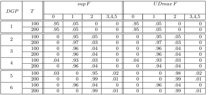
Table 2: Empirical distribution of the estimated number of breaks
sup F U Dmax F
DGP T
0 1 2 3,4,5 0 1 2 3,4,5 100 .95 .05 0 0 .95 .05 0 0 1
200 .95 .05 0 0 .95 .05 0 0 100 0 .95 .05 0 0 .95 .05 0 2
200 0 .97 .03 0 0 .97 .03 0 100 0 .96 .04 0 0 .96 .04 0 3
200 0 .96 .04 0 0 .96 .04 0 100 .04 .93 .03 0 .04 .93 .03 0 4
200 0 .96 .04 0 0 .94 .04 0 100 .03 0 .95 .02 0 0 .98 .02 5
200 0 0 .99 .01 0 0 .99 .01 100 0 .96 .04 0 0 .96 .04 0 6
200 0 0 .99 .01 0 0 .99 .01
Notes: The blocks headed sup F or UDmax F give the empirical distribution of ˆ
mT, obtained via the sequential strategy using Sup FT(1; 1) or UDmax FT(5,1) on the first step with the maximum number of breaks set to five.
good size and power properties of sup F tests; they improve as the sample size
increases, for both m = 1, m = 2, and so do the properties of the estimate for
number of breaks ˆmT in Table 2.
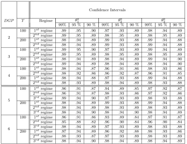
Parameter confidence interval coverages are reported in Table 3 and are in all
cases close to the nominal size. Overall, our methodology seems to work well in
finite samples.
7
An Application to the US Interest Rate
Reac-tion FuncReac-tion
Several recent theoretical and empirical studies question the assumptions of
linear-ity and/or parameter stabillinear-ity underlying (US) monetary policy rules, seeinteralia
Schaling (2004), Dolado, Mar´ıa-Dolores, and Ruge-Murcia (2004), Bec, Salem, and
Collard (2002), Kim, Osborn, and Sensier (2005), Kesriyeli, Osborn, and Sensier
Table 3: Empirical coverage of parameter confidence intervals
Confidence Intervals
θ0
1 θ02 θ30
DGP T Regime
99% 95 % 90 % 99% 95 % 90 % 99% 95 % 90 % 100 1st regime .99 .95 .90 .97 .93 .89 .98 .94 .89
2ndregime .99 .95 .89 .98 .95 .89 .98 .95 .89
2
200 1st regime .98 .94 .89 .99 .93 .88 .99 .94 .88
2ndregime .98 .94 .89 .99 .93 .88 .99 .94 .88
100 1st regime .99 95 .90 .97 .93 .89 .99 .94 .89
2ndregime .99 .95 .89 .98 .95 .89 .98 .95 .89
3
200 1st regime .98 .94 .89 .98 .94 .89 .99 .94 .90
2ndregime .99 .94 .89 .98 .94 .89 .98 .94 .90
100 1st regime .98 .94 .87 .96 .91 .86 .98 .93 .86
2ndregime .98 .92 .86 .96 .92 .87 .96 .91 .85
4
200 1st regime .98 .94 .88 .97 .93 .88 .99 .94 .88
2ndregime .98 .93 .89 .98 .94 .89 .98 .93 .88
100 1st regime .96 .91 .87 .94 .89 .85 .97 .92 .87
2ndregime .96 .91 .87 .98 .93 .86 .97 .92 .86
3rd regime .99 .94 .90 .97 .93 .89 .98 .93 .88
5
200 1st regime .98 .94 .89 .99 .93 .88 .99 .94 .88
2ndregime .98 .94 .89 .98 .93 .89 .98 .93 .89
3rd regime .98 .94 .90 .98 .94 .90 .98 .94 .89
100 1st regime .96 .91 .86 .93 .89 .84 .97 .91 .87
2ndregime .95 .88 .82 .96 .90 .84 .96 .90 .84
3rd regime .98 .94 .89 .97 .93 .89 .98 .93 .88
6
200 1st regime .97 .94 .89 .96 .92 .88 .98 .93 .86
2ndregime .98 .93 .87 .97 .93 .89 .98 .93 .89
3rd regime .98 .94 .90 .98 .94 .89 .98 .94 .89
Notes: The column headed 100a% gives the percentage of times the 100a% confi-dence intervals for each parameter contains its true value.
In most of these studies, nonlinearity is modeled via switching regimes,
thresh-old behavior or as a smooth transition between (linear) regimes associated with
different inflation gaps (deviations of inflation from target), output gaps
(devia-tions of output from their potential) or both.
Threshold models are largely viewed today as a special case of smooth
transi-tion models, when the smoothness parameter of the transitransi-tion functransi-tion approaches
infinity. Similarly, change-point models are viewed as a special case of smooth
transition models with the state variable time and the smoothness parameter
such a treatment is not desirable, since it is difficult to develop estimation and
inference theory in the presence of parameters approaching infinity; even if these
parameters are not the main object of inference, it is likely that their estimation
will affect the estimation of other parameters of interest. While this discussion
highlights the importance of distinguishing between breaks and time transitions
with smoothness parameters close to infinity, it does not preclude the treatment of
smooth and sudden change jointly. Our methodology allows for such a treatment,
since a large class of smooth transition models are estimated via NLS and are
thus nested by our model. Structural stability in these models can be assessed
via the testing strategies we proposed. If there is evidence of change points, our
methodology allows for modeling them jointly with nonlinearity.
To illustrate this point, we revisit the nonlinear model of the US federal funds
rate reaction function considered in Kesriyeli, Osborn, and Sensier (2006). Unlike
the tests proposed by Eitrheim and Ter¨asvirta (1996), our tests are designed
specif-ically against the alternative of structural change, providing further evidence of
parameter nonconstancy in the model employed by Kesriyeli, Osborn, and Sensier
(2006).
Following evidence of nonlinearity and structural change, Kesriyeli, Osborn,
and Sensier (2006) use monthly data from 1984 : 1-2002 : 12 to model the US
interest rate reaction function, employing the following two-transition model:
rt=x′tβ1+xt′β2G1(∆3rt−1;γ1, c1) +x′tβ3G2(t;γ2, c2) +ut
with rt is the federal funds rate,x′
t = (1, rt−1, rt−2, πgt−1, πgt−2, πgt−3, ogt−1, ogt−2,
∆wcpt−3), where πgt and ogt denote inflation gap, respectively output gap, while
∆wcpt stands for the change in the world commodity prices at time t.11 Here,
G1(∆3rt−1; γ1, c1) is a logistic transition function associated with a three month
11For details on how these series are constructed at a monthly frequency, see Kesriyeli, Osborn,
change in the interest rate, i.e. st,1 = ∆3rt−1 =rt−1−rt−4, andG2(t;γ2, c2) another
logistic transition function associated with time, i.e. st,2 =t:
Gi(st,i;γi, ci) ={1 + exp[−γi(st,i−ci)/σˆ(st,i)]}−1, i= 1,2
This model is routinely estimated via NLS, and the smoothness Assumption 3
implicitly holds. The properties of a logistic transition function ensure that the
moment conditions in Assumption 4 are satisfied, as long as the implied moments of
regressor and error distribution exist. Assumptions prone to violation are possibly
Assumptions 1(i),(ii), 6. Potential violations are discussed at the end of this
section.
In this model, Kesriyeli, Osborn, and Sensier’s (2006) obtain a large estimate of
the time smoothness parameter (γ2 = 1082, t-value 0.02) which could be indicative
of a break rather than a smooth transition. This is confirmed by a time-transition
function that lasts only one period. Hence, there is scope to use our tests to detect
potential change-points. However, since Kesriyeli, Osborn, and Sensier’s (2006)
potential ‘break’ occurs at the beginning of the sample, we test for breaks by
enlarging the sample to 1982 : 7−2002 : 12.12 Because of adding observations, the
model specification may change, an issue which we address by step-wise recreating
the model specification strategy in Kesriyeli, Osborn, and Sensier (2006).
This strategy involves first selecting a linear model, then assessing the adequacy
of this specification by performing on this model separate tests for parameter
instability and neglected nonlinearity, and finally using the results from these
tests to inform their final model specification. Following the same steps, we start
with a linear stable model specification, and by backward selection via AIC and
12Our dataset starts at 1982 : 3, but after constructing different lags we lose 4 periods. We
BIC arrive at the following model:
rt =x′tβ+ut, with x′t = (1, rt−1, rt−2, ogt−1, ogt−3, πgt−2)
Bai and Perron’s (1998) tests indicate one possible break, at 1984:9, evidence
supported by a UDmax test (UDmax = 34.855) significant at the 1% level but
not by a sup F test (sup FT(1; 6) = 16.679), insignificant at the 10% level. On
the other hand, tests against nonlinearity proposed in Luukkonen, Saikkonen, and
Ter¨asvirta (1988) indicate possible nonlinearity related tort−1, rt−2, πgt−2, rt−4. A
single-transition model withrt−4 fits worse than one withrt−1and ∆3rt−1as a state
variable. The latter state variable is justified not only by tests and grid searches,
but also by the intuition that the Fed should reacts differently to previous positive
or negative changes in interest rates on a quarterly (thus smoother) basis.
Thus, with a slightly different model specification, we obtain the same state
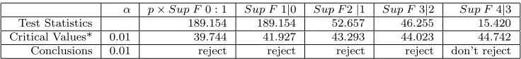
variable as in Kesriyeli, Osborn, and Sensier (2006), but find evidence of three
breaks:
rt=x′tβ1(i)+x′tβ2(i) G1(∆3rt−1;γ1(i), c (i)
1 ) +ut, t∈[Ti−1+ 1, Ti] i= 1, . . . ,4
(16)
with x′
t = (1, rt−1, rt−2, ogt−1, ogt−3, πgt−2). This evidence is supported by the
[image:33.612.114.482.544.586.2]instability tests in Table 4, reported for a cut-off ǫ= 0.10.
Table 4: Stability Tests and Critical Values
α p×Sup F0 : 1 Sup F1|0 Sup F2|1 Sup F3|2 Sup F4|3 Test Statistics 189.154 189.154 52.657 46.255 15.420 Critical Values* 0.01 39.744 41.927 43.293 44.023 44.742 Conclusions 0.01 reject reject reject reject don’t reject *Critical values forp= 14 forǫ= 0.10 andα= 0.01 are taken from Hall and Sakkas (2010).
The Akaike information criterion (AIC) in Table 5 confirms that a model with
Table 5: AIC and BIC of the Estimated Models
Model SS AIC BIC Linear 18.154 -2.558 -2.471 STAR One Transition,m= 0 16.771 -2.572 -2.372 STAR Two Transitions∗
,m= 0 11.640 -2.872 -2.559 STAR One Transition,m= 1 8.977 -3.067 -2.639 STAR One Transition, Restricted∗∗
,m= 1 11.707 -2.866 -2.553 STAR One Transition,m= 2 7.007 -3.201 -2.574 STAR One Transition,m= 3 5.585 -3.305 -2.465
∗
The second state variable is time∗∗
[image:34.612.109.493.241.393.2]Restriction refers to the transition function parameters not breaking across regimes.
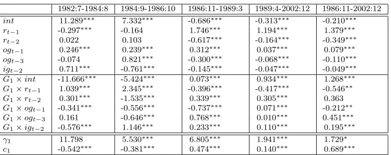
Table 6: Estimates for Two and Three Breaks
1982:7-1984:8 1984:9-1986:10 1986:11-1989:3 1989:4-2002:12 1986:11-2002:12
int 11.289∗∗∗
7.332∗∗∗
-0.686∗∗∗
-0.313∗∗∗
-0.210∗∗∗
rt−1 -0.297∗∗∗ -0.164 1.746∗∗∗ 1.194∗∗∗ 1.379∗∗∗
rt−2 0.022 0.103 -0.617∗∗∗ -0.164∗∗∗ -0.349∗∗∗
ogt−1 0.246∗∗∗ 0.239∗∗∗ 0.312∗∗∗ 0.037∗∗∗ 0.079∗∗∗
ogt−3 -0.074 0.821∗∗∗ -0.300∗∗∗ -0.068∗∗∗ -0.110∗∗∗
igt−2 0.711∗∗∗ -0.761∗∗∗ -0.145∗∗∗ -0.047∗∗∗ -0.049∗∗∗
G1×int -11.666∗∗∗ -5.424∗∗∗ 0.073∗∗∗ 0.934∗∗∗ 1.268∗∗∗
G1×rt−1 1.039∗∗∗ 2.345∗∗∗ -0.396∗∗∗ -0.417∗∗∗ -0.546∗∗
G1×rt−2 0.301∗∗∗ -1.535∗∗∗ 0.339∗∗∗ 0.305∗∗∗ 0.363
G1×ogt−1 -0.341∗∗∗ -0.556∗∗∗ -0.737∗∗∗ 0.071∗∗∗ -0.212∗∗
G1×ogt−3 0.161 -0.646∗∗∗ 0.768∗∗∗ 0.010∗∗∗ 0.451∗∗∗
G1×igt−2 -0.576∗∗∗ 1.146∗∗∗ 0.233∗∗∗ 0.110∗∗∗ 0.195∗∗∗
γ1 11.798 5.530∗∗∗ 6.805∗∗∗ 1.941∗∗∗ 1.729∗
c1 -0.542∗∗∗ -0.381∗∗∗ 0.474∗∗∗ 0.140∗∗∗ 0.689∗∗∗
with no breaks, as well as to a linear model.13 The global estimates of the three
breaks are located at 1984:8, 1986:10 and 1989:3, all with tight confidence bounds
of only one-period before and after.
Residual and residual autocorrelation plots do not show evidence of
autocor-relation (Ljung-Box test p-value: 0.1649) or unit roots (Augmented Dickey-Fuller
test p-value: 0.0001). Thus, the model in (16) admits a Markov-chain
representa-tion, and Assumption 1(i) is satisfied if{yt, xt, ut}is assumed ergodic within each
regime.14 Hence, Assumption 1 is plausible.
13According to the Bayesian information criterion (BIC), one would pick only one break, but
this is in contrast to both AIC and the outcome of the stability tests, so we pick a model with three breaks.
14Ergodicity is a common assumption for smooth transition models. For sufficient conditions,
Moreover, Bai and Perron’s (1998) tests on the squared residuals, UDmax =
4.375;sup F(1|0) = 1.555, do no reject at the 10% level, indicating no breaks
in variance, and there does not seem to be much evidence of
heteroskedastic-ity. Hence, Assumption 6(i)-(ii) seems to hold. On the other hand, Assumption
6(iii)-(iv), could be violated, e.g. if, according to Hansen (2000), there are breaks
in the marginal distribution of the regressors. Any arguments related to
Vol-cker’s disinflation inducing a break in the mean of the inflation gap are refuted
by UDmaxFT(5,6) = 1.244, sup FT(1 :p) = 0.044, both insignificant at the 10%,
perhaps due to few observations before disinflation was completed. There could
be breaks in the volatility of output gap, consistent with the ’Great Moderation’
dated by Stock and Watson (2002) around 1984 (even though these are breaks in
conditional variances of an AR process modeling output growth). Since this
po-tential break is at the beginning of the sample and it does not affect consistency of
break-point estimates, the power of tests is not affected; the size of the sequential
test F(3|2) may be affected, but one can run Wald tests instead.15
Table 6 shows the estimates we obtain in the various regimes. The conclusions
of the period 1989:4-2002:12 are similar to Kesriyeli, Osborn, and Sensier’s (2006)
findings with respect to different regimes, since we obtain a similar threshold.
However, we find evidence of more than one break; additional breaks are suggested
in Kesriyeli, Osborn, and Sensier (2006) by an Eitrheim and Ter¨asvirta (1996)
parameter constancy test p-value of 0.042, but our sequential sup F-test, designed
specifically against for breaks, detects them at the 1% level. We find that the first
break occurs close to the one found in Kesriyeli, Osborn, and Sensier’s (2006), and
can be linked to recovery from the deep recession of 1981-1982, start of Reagan’s
second term and Volcker’s era of disinflation. We also find that the period
1989:4-the 1% critical value boundary, so one could pick three regimes instead of four. From Table 6, one can note from the small smoothness parameter that the third regime is close to linear; in the latter case, ergodicity is no longer of concern.