http://dx.doi.org/10.4236/opj.2016.67019
Characterization of a Multimodal and
Multispectral Led Imager: Application to
Organic Polymer’s Microspheres
with Diameter
Φ
= 10.2
μ
m
Marcel A. Agnero
1,2, Jérémie T. Zoueu
1, Kouakou Konan
11Laboratoire d’Instrumentation d’Image et Spectroscopie, Institut National Polytechnique Félix
Houphouët-Boigny, Yamoussoukro, Côte d’Ivoire
2Laboratoire de Physique de la Matière Condensée et Technologie, University Félix Houphouët-Boigny, Abidjan,
Côte d’Ivoire
Received 25 May 2016; accepted 18 July 2016; published 21 July 2016
Copyright © 2016 by authors and Scientific Research Publishing Inc.
This work is licensed under the Creative Commons Attribution International License (CC BY). http://creativecommons.org/licenses/by/4.0/
Abstract
conven-tional instrument.
Keywords
Multispectral Imaging, Reference Wavelength, Correction Coefficients, Modulation Transfer Function
1. Introduction
Multispectral microscopy establishes a link between spatial and spectral information resulting from light-matter interaction. It can be described as spectroscopy and microscopy coupler. This technique is well established in remote sensing and satellite imagery areas. It is now extended to the microscopy area because of its various ad-vantages.
Several works illustrate the importance of multispectral microscopy. Zoueu et al. [1] have shown that using multispectral imaging allows detecting malaria without using fluorescent labels for parasites as it is the case of thick and thin blood smears. Multispectral imaging is an important tool in the delimitation of reserved forests [2]
and also in agriculture framework for rapid detection of fruit diseases [3][4].
Several multispectral imaging technologies, in spite of their high cost, are used in the sequential or parallel acquisition of images of the same scene using different wavelengths and generate an optical spectrum associated to any pixel in the image [5]. Progresses are observed in the implementation of low cost multi spectral imaging devices. Merdasa et al. [6] have modified a classical microscope where the white source is replaced by quasi monochromatic sources and adapted to multispectral imaging device to detect malaria. But the microscope is li-mited to five spectral channels (wavelengths) in the visible spectral range. Increasing the number of spectral channels in the visible spectrum and expanding channel acquisition to the light that is outside the sensitivity of the human eye offer several advantages. Mikkel Brydegaard et al. [2] have constructed a multispectral micro-scope with a large spectral band ranging from ultraviolet to near-infrared wavelengths, active in transmission mode and which allows an information enhancement in the study of specimen.
In such a system, the spectral information reconstruction requires images of acceptable quality (sharp and of the same scale). But, using a large spectral band induces the variation of focal plan position of the imager due to the phenomenon of chromatic aberration which affects the quality of the images. This is a major problem met in multispectral imaging. To reduce distortion due to chromatic aberration, reflex objective can be used such as Cassgrain objective [7]; a two-lens system or an apochromatic triplet equips some systems to reduce curvature of the image and to minimize residual aberrations in the focal plane [8][9]. The method of refocusing focal plan of the multispectral device can be done at each spectral channel [10]. This solution can introduce a geometrical offset on one hand and slow down the acquisition protocol of the imaging system on the other hand.
In the present work, a low cost multimode multispectral microscope with Cassgrain objective using a camera and a set of monochromatic Light Emitting Diodes (LEDs) as illumination sources was constructed and we present a new approach to calibrate that instrument to be a standard one. By calibration, we mean:
- the determination of the wavelength used to fix its focal plan where the phenomenon of chromatic aberration is more reduced,
- the correction of the extracted spectra from the images making them in agreement with the standards spectra, - the determination of modulation transfer function which is an important tool in an imager’s characterization, - the evaluation of its capacity to recognize the specimen’s properties.
For this purpose, we used it to make measurements on samples with well-known properties such as homoge-neous filters and organic polymer’s microspheres (latex) with diameter
Φ =
10.2 m
µ
before using it on speci-men with unknown properties. Measurespeci-ments were done in transmission mode, reflection mode and scattering mode. Results are analyzed using multivariate analysis methods.2. Materials and Methods
2.1. Multi Spectral Device’s Description
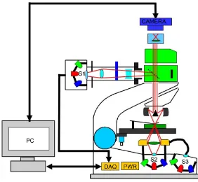
Figure 1. Multimodal and multispectral microscope setup. S1, S2 and S3 are a set of LED light sources for reflection, transmission and scattering modes
re-spectively. The red lines illustrate the beam path interacting with the specimen.
improved version of the LED multispectral microscope built by Brydegaard et al. [2], adapted and descripted by Zoueu et al. [7].
The light sources S1, S2 and S3 are controlled via a data acquisition (DAQ) connected to a computer (PC). All are controlledby a LabView (Lab View 8.6, licence no. M 74 × 11278) operation code. Each light source is a set of quasi-monochromatic Light Emitting Diodes (LEDs) with the following spectral band: 375 nm, 400 nm, 435 nm, 470 nm, 525 nm, 590 nm, 625 nm, 660 nm, 700 nm, 750 nm, 810 nm, 850 nm, 940 nm. Before any measurement, we need to align all the optics. All The measurements are done in the darkness to minimize back ground light.
2.2. Measurement’s Procedure
Measurements are made on two types of samples:
-Filters, used as homogeneous samples whose standard spectra are extracted from the spectrometer (Compact Spectra Suite Ocean Optics USB4000).
-Organic polymer’s microspheres (latex) with diameter
Φ =
10.2 m
µ
whose properties are known. There are the homogeneity, the isotropicity and the spherical geometry.The microspheres’ samples are prepared on slides made of the highest purity, corrosion-resistant glass with dimensions 75 mm × 25 mm × 1 mm. The measure in each mode (transmission, reflection or scattering) needs three types of images acquired in the same acquisition conditions:
-The image Ts, Rs or Ss if it’s about transmittance’s measure, reflectance’s measure or scattering’s measure respectively. That image contains noise due to the parasite light in the dark environment and to the set-up electronic system;
-The image Td, Rd or Sd is due to noise respectively in transmission mode, reflection mode or scattering mode;
-The image Tb, Rb or Sb is for the reference in transmission mode, reflection modes or scattering mode respectively.
measurement. The measurement is an automated acquisition of thirteen images from the same scene and each image corresponds to a wavelength of illumination. The wavelengths selection as reference is part of the goals of this study.
In the transmission mode, we active the geometry “brightfield” as indicated on the interface presented by Lab view operation code. The signal Ts is measured after having put the slide containing the sample on the micro-scope’s holder. The reference signal Tb in the transmission mode is measured by maintaining the same slide on the microscope’s holder so that an image of the around area of the sample is acquired. For the measure of Td, the microscope’s holder is kept empty and the electric battery for the different LEDs is set off to avoid eventual il-lumination of the camera. In order to rise up the acquisition speed, we establish a measurement protocol, that’s to say we acquire one of the signals Ts, Tb or Td in a specific condition; this condition constitutes the protocol we call through our operation code to acquire the two other signals.
The corrected image T of the sample is given by the relation (1):
s d b d T T T T T − =
− . (1)
In the measurement of the reflectance, the alignement of optics in the microscope and fixation of its focal plan at the reference wavelength being done during the measures in transmission mode, we active the geome-try ”reflection” inthe Lab view code interface in order to run the automated acquisition of the thirteen images.The signal Rs ismeasuredafter having put the slide containing the sample on the microscope’s holder.The signal
b
R is acquiredby usinga diffuser in the place of the sample, with its white face upin the microscope. The diffuser eliminates dissymetry light dispatching andallows anuniform intensity distributionin the camera’s field of theview
[3]. To acquire the image, Rd, the microscope’s holder is kept empty in order to get parasite reflection dueto the opticsin the microscope. The corrected image R of the sample is given by the relation (2) [3]:
s d b d R R R R R − =
− . (2)
In scattering mode, the geometry “darkfield” is activated to run the automated acquisition of the thirteen im-ages. The signal Ss is measured after having put the slide containing the sample on the microscope’s holder. The signal Sb is measured by using a diffuser in the place of the sample, with its white face down in the microscope. To get the imageSd, we put an empty slideon the microscope’s holder.The corrected image S of the sample is given by the relation (3):
s d b d S S S S S − =
− . (3)
3. Results and Discussion
3.1. Choice of Reference Wavelength
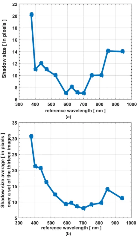
compar-ison. Each wavelength chosen as a reference defines a focal plan. In each set of the thirteen images acquired af-ter the choice of the reference, there’s only one image which is well contrasted. Indeed, this image is acquired with light source used to fix the focal plan. Then, we have thirteen contrasted images, each one corresponding to a reference wavelength. First, we compare these thirteen contrasted images to appreciate that presenting more reduced shadow. This comparison highlights that the reference wavelengths 590 nm, 625 nm, 660 nm and 700 nm are the ones whose corresponding images present more reduced shadow spreading on 7 pixels, 8,06 pixels, 7,07 pixels and 7 pixels respectively (Figure 2(a)). In second time, we determine the mean of the shadow size over the images from each set. The comparison shows in Figure 2(b) that the reference wavelengths 590 nm, 625 nm, 660 nm, 700 nm and 750 nm are the ones whose corresponding set of images present more reduced shadow spreading on 9.31 pixels, 9.67 pixels, 8.66 pixels, 8.01 pixels and 9.14 pixels respectively.
The first comparison shows that fixing the focal plan with the reference 590 nm or 700 nm, the microsphere’s image observed at the wavelength 590 nm or 700 nm respectively, present more reduced shadow (Figure 2(a)).
[image:5.595.199.428.259.652.2]The second comparison reveals that only with the reference 700 nm, the microsphere’s images acquired using the set of the thirteen wavelengths present in average more reduced shadow (Figure 2(b)). These two types of
Figure 2. (a) Shadow size of each contrasted image correspond-ing to a reference wavelength, a contrasted image is an image acquired with a wavelength (light) used to fix the focal plan of the microscope, this wavelength is called reference wavelength; (b) Shadow size average over each set of the thirteen images,
comparison allow to select 700 nm as the best reference wavelength to fix the focal plan of the multi spectral microscope.
3.2. Spectra Extraction and Correction Coefficients
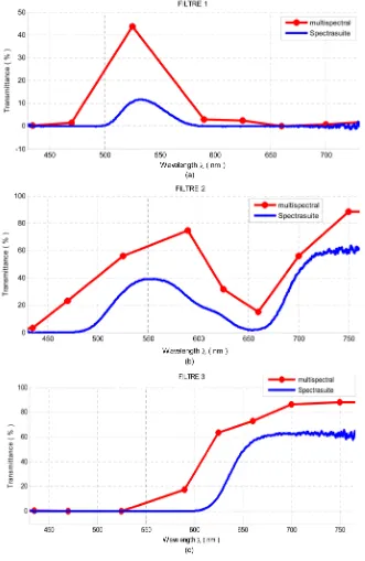
[image:6.595.149.480.176.685.2]The images acquired from different filters (filter 1, filter 2 and filter 3) with the microscopeled to the extraction of their spectra in transmission and reflection modes. Figure 3 and Figure 4 present a comparison of these spectra
Figure 3. Transmittance Spectra for filter 1 (a), for filter 2 (b), for filter 3 (c), extracted by the standard spectrometer Spectra Suite (spectra in blue colour) and by the multi spectral
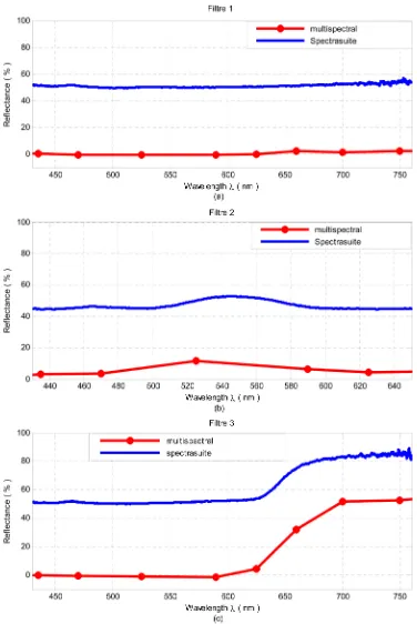
Figure 4. Reflectance Spectra for filter 1 (a), for filter 2 (b), for filter 3 (c), extracted by the standard spectrometer Spectra Suite (spectra in blue colour) and by the multi spectral microscope (spectra in red colour).
profile which indicates the nature of the different filters (filters 1, 2 and 3 are respectively pass-band, pass-band and pass-high, pass-high) but do not coincide. The filters transmit more and reflect less light than in the case we use the multi spectral microscope. So, we need to suggest a correction and make spectra in well agreement. The pixel intensity Ip from a spectral channel (p) is the contribution of the source of illumination Ep
( )
λ , the spectral sensibility S( )
λ of camera and the standard spectrum f( )
λ of the specimen. The intensity Ip, in absence of fluorescence is given by the Equation (4) [2][11]:( ) ( ) ( )
0 d
p p
I =
∫
∞E λ f λ S λ λ. (4)The thirteen wavelengths ranging from 375 nm to 940 nm give thirteen spectral channels (p). λ takes the different values of emission spectral band of the LED. The spectra are discrete because they are built on thirteen points joint through Matlab. The points represent intensity Ip of a pixel in function of the positions of the picks for the spectral emission of the LEDs. The intensity Ip in a pixel is an average taken over an emission spectral band of a quasi-monochromatic LED source. This causes a discrepancy between the spectra obtained from the multi spectral microscope and the standard spectra [12].
The transfer function Tp
( )
λ of system in each spectral channel is derived from the formula (4) [12]:( )
( ) ( )
p p p
T λ =τ E λ S λ . (5)
p
τ is a constant chosen to normalize Tp
( )
λ over the passband of the channel (p).The Equation (4) does not take into account the imperfection of the optics in the multi spectral device. That induces discrepancy between the constructed spectra and the standard spectra. Chromatic aberration, eventual fluorescence of the specimen and camera shot noise also induce this discrepancy [2]. Beside these causes, the non-monochromaticity of the LEDs contributes to the discrepancy. Indeed, if ∆p is the size of the pass band for a spectral channel (p) around which Taylor development of standard spectrum f
( )
λ is made, the Equation (4) becomes [12]:( )
1 ( )( )
! p( )
(
)
dn
n
N p
p p n p p
f
I f T
n
λ
λ = ∆ λ λ λ λ
= +
∑
∫
− . (6)We can see easilythe contribution for the LED’s non-monochromaticity to the discrepancy. Figure 3 shows that the discrepancy tends to disappear when the standard transmittance tends toward zero value. It appears when the standard transmittance rises up. This variation reveals that the standard and multi spectral transmit-tances can be linked through this linear relation:
t st msp msp
T =
α
T . (7)msp
T is the transmittance spectrum got from the multi spectral microscope; Tst is the standard transmittance spectrum;
α
mspt is the standardization coefficient for transmittance got from multi spectral device. It’s an av-erage obtained over the spectral band where discrepancy exists and over the three filters.From spectra presented in Figure 3, we deduced
α
mspt =0.3833. The relation (7) becomes:0.3833
st msp
T = T . (8)
Figure 4 presents the measures of reflectance and shows that the standard and multi spectral reflectance can be linked through this relation (9).
r st msp msp
R =
α
R (9)msp
R is the reflectance spectrum got from the multi spectral microscope; Rst is the standard reflectance spectrum;
α
mspr is the standardization coefficient for reflectance got from multi spectral device. It’s an aver-age obtained over the spectral band and over the three filters (Figure 4). We highlight the reflectance spectra variation through the following Table 1 which suggests the mean valueα
mspr given by the relation (10):56.3344 if 1.5%
12.2114 if 1.5% 10%
2.7059 if 10%
msp r msp msp msp R R R α ≤
= < <
≥
Table 1. Reflectance spectra variation for the different filters presented in term of values allowing the determination of
r msp
α .
Filters Reflectance extracted from multi spectral device Reflectance extracted from standard spectrometer
1 and 3 Lower than 1%, 5% Quasi-constant close to 50%
2 Included between 1%, 5% and 10% Included between 45% and 53%
3 Higher than 10% Included between 55% and 85%
3.3. Determination of the Modulation Transfer Function
The modulation transfer function (FTM) is an important tool allowing to quantify an image quality. It expresses the imager’s capacity to transmit information from a scene in spatial frequency domain and determines its reso-lution. In this work, the FTM of our multi spectral imager in transmission mode is evaluated through the edge method [13]. The algorithm for the determination of the FTM consists of the following steps [14]:
- acquisition of an image of a tilted edge, - determination of the edge spread function ESF,
- differentiation of the ESF to obtain the line spread function LSF, - calculation of the Fourier Transform of the LSF to obtain the FTM.
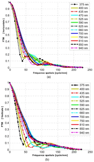
For each illumination source, we evaluated the modulation transfer function following the lines and columns of the imager (Camera pixel size: 2.2 µm × 2.2 µm) called respectively horizontal FTM and vertical FTM (Figure 5).
The decrement of FTM for high spatial frequencies shows that our device behaves like a low-pass filter and transmits more details in low spatial frequency band. This decrement depends on the illumination wavelength used. Using the wavelength 375 nm, the decrement of the corresponding FTM (in low spatial frequency band) is the most quick but, as we use the wavelength 700 nm, the decrement of the corresponding FTM is less quick. This confirms that images acquired with 700 nm as illumination wavelength are more contrasted whereas the images acquired with 375 nm contain less detail.
3.4. Application to Organic Microspheres
After the determination of correction coefficients, the multi spectral microscope is used to make measurements on organic polymer’s microspheres of diameter
Φ =
10.2 m
µ
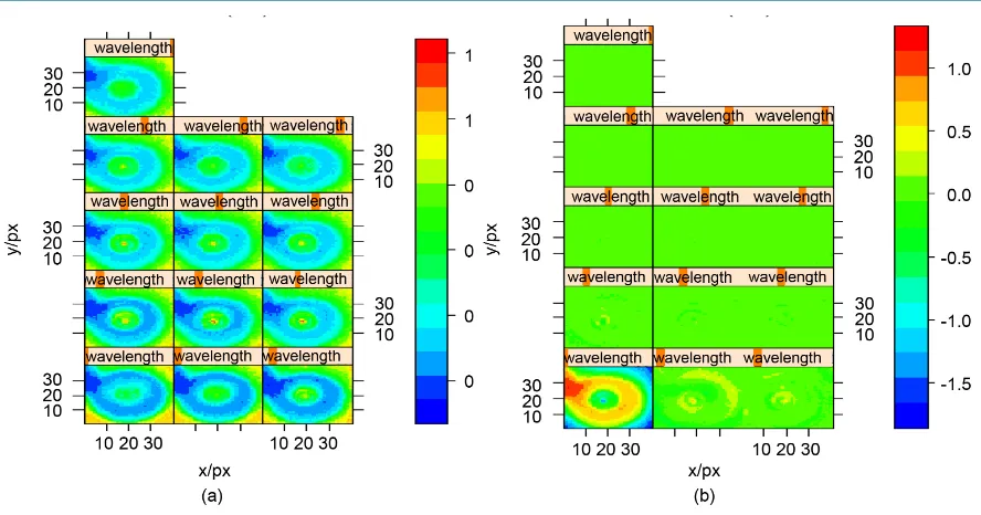
with known properties (homogeneity, isotropici-ty and spherical geometry). The different measures are treated through multivariate analysis methods such as principal component analysis (PCA), k-means method [15]-[22].If a sample of three objects of colors red, green and blue is illuminated using red-light, only the red object will be observed. If it is illuminated using green light, only the green object will be seen. If it’s illuminated by blue light, only the blue object will be observed. So, each wavelength reveals specific information about the speci-men. Figure 6(a) presents a spectral representation of microsphere’s images in transmission mode for the thir-teen spectral channels corresponding to the different illumination wavelengths. In Figure 6(a), we can see thir-teen images which seem to be identical; it means there’s a repetition of informations from a spectral channel to another. The analysis of these spectral images using PCA allows to isolate informations [15]-[18]. Applying PCA to the spectral images data (Figure 6(a)), we condense informations into new group so that they do not present any correlation between them and are ordered in terms of the percentage of variance giving more infor-mations (Figure 6(b)). We observe that all the informations are quasi located into the first principal component (Figure 6(b)). Therefore, the PCA means that only one spectral channel or one illumination wavelength is suffi-cient to describe the microsphere. So, our multi spectral device confirms that the microsphere effectively is con-stituted of identical elements; that is to say it’s well homogeneous and isotropic.
Figure 5. Modulation transfer function horizontally (a) and vertically (b) of the
multi spectral imager for different quasi-monochromatic illumination sources.
( )
22(
(
)
)
22(
(
)
)
sin tan
0.5
sin tan
i t i t
i
i t i t
R α α α α α
α α α α
− −
= × +
+ +
. (11)
i
α and αt are respectively incidence angle and refraction angle and R is the Reflection.
Figure 6. Spectral intensity distribution inside the microsphere in transmission mode, presented for the thirteen spectral channels (375, 400, 435, 470, 525, 590, 625, 660, 700, 750, 810, 850 and 940) in nm, starting from the bottom on the left to the top, as indicated by the orange lines (a); the new group of principal component images (PCs images) where informations are isolated using principal components analysis is presented in (b). The PCs images start by PC1 on the bottom on the left to
the top as indicated by the orange lines.
Figure 7. Intensity dispatching in the microsphere image presented by k-means method.
4. Conclusion
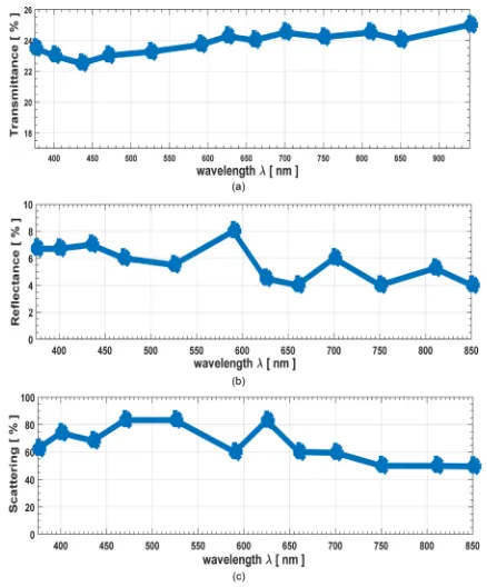
[image:11.595.189.441.377.564.2]Figure 8. Standardized spectrum in transmission mode (a), standardized spectrum in reflection mode (b) and non-
standardized spectrum in scattering mode (c), extracted from microsphere by the multi-spectral microscope.
has confirmed its homogeneity. Through K-means method, the experimental instrument recognized the spheric-ity of the microsphere. This led to the extraction of the standard transmittance and reflectance spectra. Therefore, this microscope is used as a routine instrument.
References
Multis-pectral Imaging Applied to Plasmodium Diagnosis. Journal of Applied Sciences, 8, 2711-2717. http://dx.doi.org/10.3923/jas.2008.2711.2717
[2] Brydegaard, M., Guan, Z. and Samberg, S. (2009) Broad-Band Multi-Spectral Microscope for imaging Transmission Spectroscopy Employing an Array of Light-Emitting Diodes (LEDs). American Journal of Physics, 77, 104-110. http://dx.doi.org/10.1119/1.3027270
[3] Sangare, M., Tekete, C., Bagui, O.K., Ba, A. and Zoueu, J.T. (2015) Identification of Bacterial Diseases in Rice Plants Leaves by the Use of Spectroscopic Imaging. Applied Physics Research, 7, 61-69.
http://dx.doi.org/10.5539/apr.v7n6p61
[4] Sangare, M., Agneroh, T.A., Bagui, O.K., Traore, I., Ba, A. and Zoueu, J.T. (2015) Classification of African Mosaic Virus Infected Cassava Leaves by the Use of Multi-Spectral Imaging. Optics and Photonics Journal, 5, 261-272. http://dx.doi.org/10.4236/opj.2015.58025
[5] Levenson, R. and Mansfield, J. (2006) Multispectral Imaging in Biology and Medicine: Slices of Life. Cytometry Part A, 69A, 748-758. http://dx.doi.org/10.1002/cyto.a.20319
[6] Merdasa, A., Brydegaard, M., Svanberg, S. and Zoueu, J.T. (2013) Staining-Free Malaria Diagnostics by Multispectral and Multimodality Light-Emitting-Diode Microscopy. Journal of Biomedical Optics, 18, Article ID: 036002.
[7] Zoueu, T. and Tokou, S. (2012) Trophozoite Stage Infected Erythrocyte Contents Analysis by Use of Spectral Imaging LED Microscope. Journal of Microscopy, 245, 90-99. http://dx.doi.org/10.1111/j.1365-2818.2011.03548.x
[8] Strojnik, M., Wang, Y., Randolph, J.E. and Ayon, J.A. (1991) Site-Certification Imaging Sensor for the Exploration of Mars. Optical Engineering, 30, 590-597. http://dx.doi.org/10.1117/12.55842
[9] Strojnik, M., Wang, Y. and Paez, G. (1995) Design of a High-Resolution Telescope for an Imaging Sensor to Charac-terize a (Martian) Landing Site. Optical Engineering, 34, 3222-3228
[10] Rueda, L. (2014) Microarray Image and Data Analysis Theory and Practice. Electrical Engineering/Computer Science, 301-303.
[11] Ohta, N. (1981) Maximum Errors in Estimating Spectral-Reflectance Curves from Multispectral Image Data. Journal of the Optical Society of America, 71, 910-913. http://dx.doi.org/10.1364/JOSA.71.000910
[12] Stephen, K. and Friedrich, O. (1977) Estimation of Spectral Reflectance Curves from Multispectral Image Data. Applied Optics, 12, 3107-3114.
[13] Estribeau, M. ( 2004) Analyse et modélisation de la fonction de transfert de modulation des capteurs d’images à pixels actifs CMOS, Thèse de Doctorat, Ecole Nationale Supérieure de l’Aéronautique et de l’Espace.
[14] Egbert, B., Susanne, G. and Ulrich, N. (2003) Simple Method for Modulation Transfer Function Determination of Dig-ital Imaging Detectors from Edge Images. Proceedings of SPIE, 5030, 877-884.
http://dx.doi.org/10.1117/12.479990
[15] Urska, D., Paul, H., Chris, B., Stewart, A. and Sean, M. (2011) Principal Component Analysis on Spatial Data: An Overview. Annals of the Association of American Geographers, 103, 1-23.
[16] Barry, M. and Paul, G. A Brief Introduction to Multivariate Image Analysis (MIA).
http://www.eigenvector.com/Docs/MIA_Intro.pdf
[17] Besse, P.C. (1992) PCA Stability and Choice of Dimensionality. Statistics & Probability Letters, 13, 405-410. http://dx.doi.org/10.1016/0167-7152(92)90115-L
[18] Analyse en composantes Principales. http://fr.wikipedia.org/wiki/Analyse_en_composantes_principales
[19] Shlens, J. (2014) A Tutorial on Principal Component Analysis.
[20] Eric, W. (2014) K-Means Clustering Algorithm from Wolfram Mathworld.
[21] DUNOD. Statistique exploratoire multidimensionnelle. 3e Edition, 155-158.
[22] Bloch, I. ( 2003) Classification et reconnaissance des formes. 17.
Submit or recommend next manuscript to SCIRP and we will provide best service for you:
Accepting pre-submission inquiries through Email, Facebook, LinkedIn, Twitter, etc. A wide selection of journals (inclusive of 9 subjects, more than 200 journals) Providing 24-hour high-quality service
User-friendly online submission system Fair and swift peer-review system
Efficient typesetting and proofreading procedure
Display of the result of downloads and visits, as well as the number of cited articles Maximum dissemination of your research work