Load Balanced Geographic Routing In Wireless Sensor Networks

©IJRASET 2015: All Rights are Reserved

911

Load Balanced Geographic Routing In Wireless

Sensor Networks

S.S.Aravinth1, K.Ravikumar2, D.R.Sudharsan3, N.Vasanth4, R.J.Vigneswaran5 1

AP/CSE/ Knowledge Institute of Technology, Salem 2

ASP/CSE/ Knowledge Institute of Technology, Salem

3,4,5

II CSE / Knowledge Institute of Technology, Salem

Abstract: A wireless sensor network (WSN) is used to monitor environmental conditions, such as sound, pressure, temperature etc. and to simultaneously share their data via the network to the destination. They are enabling control of sensor activity. The development in wireless sensor networks is almost because of applications in military such as terrorist entering alerts, other countries soldiers’ intrusion etc. These networks are used in many consumer and industrial applications. Now-a-days the application domains of wireless sensor networks were grown widely. The olden Traditional routing algorithms generates traffic, while sending the packets to destination. Geographic routing algorithms require location information well. But the problem of collision and congestion traffic of data packets is full employed in Geographic wireless sensor networks. In this paper we present a Load Balanced Geographic Routing in Wireless Sensor Networks that mean that Greedy forwarding technique by taking not only considering the distance between next node and destination as single parameter for forwarding packet. But also consider and take overhead at each node. If particular node is in high load or stress then this algorithm will be used to found another option for a data transmission or packet transmission and it is also used to increase the life time of the network.

Key Terms: Wireless sensor networks, Geographical routing, Load balanced routing, Stress balancing of sensor nodes

I. INTRODUCTION

In wireless sensor networks with the traditional routing algorithms, the problem of traffic is occurred while finding the routes to the end point. Also in these networks each node requires the full topological information of the network. Geographic routing algorithms have been proved as a promising successor of ad-hoc routing techniques, because in this network it is not needed that every node to know about the network’s topology. But they suffer with the problem that traffic routed to the same region always follows the same path. This greedy forwarding approach results in consumption of more power at particular nodes which sometimes results in disconnected network. It leads to the collision & congestion problem at a particular node. We present Load Balanced Geographic Routing (LBGR) a noble approach for Routing the packet to end point. LBGR adapts Geographic routing and traffic information at each neighbour of the forwarding node for forwarding the packets.

II. ROUTING SCHEMES

A. Geographic Routing

The Initial proposals for geographic routing were simply based on greedy forwarding approaches. These algorithms even in a connected network did not guarantee a packet delivery and packet was being dropped. Since then several algorithms GPSR, GEAR and the GOAFR algorithms that are variations of compass routing have been proposed. In GPSR If the router position is known and also the destination is known the node will communicate the packet to the neighbour being closest to packet’s destination (Euclidean distance). As only neighbour and destination addresses are stored, rather than whole network, it is almost a stateless protocol. GEAR (Geographic and Energy Aware Routing) use energy aware neighbour selection for routing towards the target region.

B. Gluttonous Or Greedy Forwarding Approach

A gluttonous algorithm is one of the algorithms that is used to find the optimum path between source and destination, among all the other possible paths in a network

For example,

of steps discovery an optimal discontinuity typically requires unreasonable many steps.

C. Face Routing

In face routing a netting graph is being divided into a set of faces. A node just needs to know about immediate & close neighbours. FIGURE 2 represents how the package is routed along these faces. When surface routing starts the first way or cutting side to be traversed is in clockwise symmetry around the first point by using right-palm and fingers command to crosswise a surface. The course will be durable until fate reached. Face routing a communication is routed along the inward of the faces of the imparting graph, with surface changes at the edges intersection the S-D stripe. The ultimate routing track is shown

Figure 2

D. Relative Neighbourhood Graph

In computational geometry, the referring neighbourhood graph (RNG) is an undirected graph defined on a set of points in the Euclidean even by connecting two points p and q by an cutting side whenever there does not have being a third sharp end r that is closer to both p and q than they are to each other. Godfried discovered this relative neighbourhood graph in 1980 as a way of defining a construction from a set of points that would mate human perceptions of the form of the set. These all of above schemes of routing have bugs in a part of burden balancing in wireless sensor networks which can be overturn by the below techniques.

III. TECHNIQUES TO BALANCE LOAD OF NODE IN GEOGRAPHIC ROUTING:

A. Communication Overhead

Communication overhead is related to how much overheads or load is expected to induce at any node. The information regarding communication overhead is inferred from the node itself. Node under high stress means more traffic and therefore congestion is likely to occur. Communication overhead can be measured efficiently by four different parameters.

1) Average number of received packets: Each node has a finite memory. Number of packets the node was engaged in routing is stored at each node. This parameter gives higher priority to actual task (i.e. the actual packet routed during communication). If the count is higher than a threshold limit means node is under high stress and will suffer collision and congestion

2) Number of Neighbours: Node’s stress level depends on the neighbour count of a particular node. Obviously the node located in a dense deployment is expected to get engage in more packet transmission in geographic routing where each node want to know the data & details about their neighbour nodes. If there more number of neighbour nodes exists, then it have to store all the details of all neighbour nodes then it may leads to exceed the threshold memory limit of a n

3) Energy Level of Node: Remaining battery level can be a good signal of high communication. Lot of energy requirements signifies that node was busy in handling more request and responses. Therefore third parameter for deciding communication overhead is related with energy level of a node. As mostly, all sensor nodes start their operations with same battery level initially, therefore low battery level at any moment indicates that this node is under high stress and will most probably die soon than others.

4) Entries On Routing Table Of Each Node: This parameter is more specialized than previous two and is based on number of routing entries on each node. Entries determine with how many nodes to communicate or overhead to decide next hop. More entries means the load at the node is building up and to tackle congestion there is need of load balancing.

B. Linking

It is related to current link status between nodes which are communicating. Wireless medium with poor quality can leads to some critical problems on the communication, so parameters which indicating Wireless link status also be considered for balance load in the network. They are two parameters to find the linking status of network

1) Average Retransmission Time: There is always a time needed for transmitting the message over the link. Wireless links are a little bit unstable and communication is not so reliable over these links. Packet delivery ratio shows reliability on the communication link. These reliable communications in wireless medium retransmission schemes are generally being used to recover lost packets. An undelivered message requires retransmission. Retransmission schemes ensure the delivery of transferred message. So, there is a parameter for Status of link, average transmission time. Both queuing delay and retransmission make this value longer.

2) Average Packet Delivery Ratio: It reflects success in link characteristics and also in ratio of transmission. It is the ratio for delivered packets to destination node. High delivery ratio indicates that link is reliable and can transmit the more packets without error. Therefore, performance of network is also measured in terms of probability of packet loss.

IV. ASSUMPTION

©IJRASET 2015: All Rights are Reserved

914

A. Algorithm

The implementation of the GLBR algorithm is described into three different steps

B. Network Deployment

1) N numbers of WSN nodes are deployed randomly within a certain boundary area within a 2-Dimensional plane. N may vary from some hundred nodes to thousands nodes.

2) A node is neighbour of another node if they are separate by a distance less than their transmission range. This distance can be calculated in 2-D coordinate system by using the distance formula. If (u1,u2) are coordinate of one node and (v1,v2) are coordinate of second node, then distance between them is

D =[( ) + ( ) ]

C. Cost Estimation

Cost estimation is the distance between the node and its base station . Obviously, larger the distance and low energy results in high cost. The cost of a node to deliver packet can be calculated as used in GEAR. We will set value of tuneable weight between 0 and 1.

V. LOAD BALANCED GEOGRAPHIC ROUTING OVERVIEW

In GLBR each node will calculate its cost to deliver the packet to destination. Now while considering the load balancing parameter i.e. number of packets received node will forward the packet depending on the load at particular node. Load at particular node has 3 levels. These levels depend upon the network conditions. Large value makes the network more exposed to problems like collision and congestion. This is because in case of large values system may resist traffic variations. Small values lead to changing packet routes very frequently. Load level is mentioned by L3, L2, and L1. Each node maintains a sorted list of neighbours according to cost for delivering the packet.

ALGORITHM lbgr (T.L, N[X])

PROBLEM DESCRIPTION: // to select a correct neighbour node to transfer packets according to the load

INPUT: // Load at current node (t), total Number of nodes in network [x]

OUTPUT: // particular node where data to be transferred n[x]

If (T.L==L1) //if load is in L1 level

Choose next closest node as packet receiver

If (T.L==L2) //if load is in L2 level

Then for x=0 to nodes’ next hop list, find a node N[x] such that cost of the next node should be less than the sum of its current neighbour cost and half of the deviation in costs of forwarding node and current neighbour and load level should be L1 . Choose N[x] as the next node.

If (T.L==L3) //if load is in L3 level

For x=0 to node’s next hop list, look for a node with cost less than forwarding nodes and Load level at this node is less than L2.

First is the case when Load level is L1. At level L1 the number of packets the node was engaged in routing is very few. Packet directly will be forwarded to this node. Now, as the load level is not much higher so node is not the focus of traffic. Its cost to deliver is also comparatively less among all the neighbour. As node is engaged in routing of few packets so this level poses no problem of congestion.

Further, problem of collision is not there.

is not an intelligent move. Now suppose a node is located in a dense region and in-between to several paths lead to destination. So such a node will be engaged in routing a lot of traffic and will continue to build up. When the load for such node reaches at level L3 the situation is critical packet may got dropped, therefore switching to an alternate node is must. The condition for shifting to an alternate is that new node should have cost to deliver less than the forwarding node. Now the reason we are choosing such a node, because a node can reroute the packet to such a node that is located long from sender. So this cost of next hop should be minimum than sender it also can be avoided. In addition, load should be at level L2 or less than L2. L3 level is very problematic in this level the node is at high stress or load. Since it is engaged in routing high traffic its energy level is continuously falling and node may die out soon. This can lead to disconnection in network. Furthermore due to collision and congestion packets will drop. So retransmission will be there to provide reliable communication. This leads to delay and slow down of the network processing. By considering load (the number of packets the node was engaged in routing) collisions and congestion can be avoided.

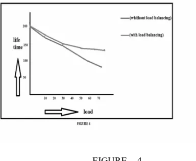
VI. RESULT

From our research we had found that by using LBGR algorithm where the load or stress that acquired by each and every node in a network can be minimized and also the life time of network is increased. This algorithm makes the life time of a network good when compared to other algorithms. It is also found that the life time of a network can be increased nearly by fifty percentages as shown in a 4th figure.

FIGURE 4

VII. CONCLUSION

A load balanced geographic routing algorithm that manage the energy and traffic at nodes in a network to achieve load balancing on densely deployed wireless networks. When compared to other algorithm this algorithm is efficient one and which increase the life time of a network. This paper makes a research and gives the brief and elaborative knowledge on, load balanced geographic routing in wireless sensor networks. This paper contains all the basics and technical things related to load balancing and also it gives a clear view on LBGR algorithm for people who really want to increase the quality and life time of network.

RFERENCES

[1] Details about geographic networks from http://en.wikipedia.org/wiki/Geographic_routing

[2] Details about routing schemes from http://ijircce.com/upload/2014/july/10_Routing.pdf

[3] Algorithm for Load balancing from www.mecs-press.org/ijcnis/ijcnis-v5-n8/IJCNIS-V5-N8-8.pdf

[4] Details about load estimation and managing from