International Research Journal of Marketing and Economics
Vol. 2, Issue 11, Nov 2015 IF- 2.988 ISSN: (2349-0314)
© Associated Asia Research Foundation (AARF)
Website: www.aarf.asia Email : [email protected] , [email protected]
BETA CALCULATION AND ROBUST REGRESSION METHODS: AN
EXAMPLE FROM THE ISTANBUL STOCK EXCHANGE
1Prof. Dr. Ali Alp2, Dr. Hakan Bilir3
2
Department of Business Administration/TOBB University of Economics and Technology, Turkey
3
Competition Authority, Turkey
ABSTRACT
Capital Asset Pricing Model (CAPM) is the most widely used method for asset valuation and
investment selection. As a systematic risk estimator, beta is the most important element of the
CAPM, and many investors trust it for selecting stocks or portfolios. The Ordinary Least
Square (OLS) is the most preferred regression method for beta calculation, indicating a
relation between stock and market index. Although the OLS is adequate in the case of normal
distribution, tail or other distribution cannot be handled successfully by the model. To
eliminate standard parametric model inefficiency, robust regression techniques have been
developed. In this paper, we propose the robust regression method Least Median Squares
(LMS) to estimate beta risk. We compare the behavior of the OLS and LMS estimation
methods using monthly returns (adjusted price for US Dollar) for firms listed on the Istanbul
Stock Exchange. Our results are also consistent with many authors’ works.
KEY WORDS: Beta Coefficient, CAPM, LMS, OLS, Robust Statistics
JEL Classification: G32
1. Introduction
The decision process of investment opportunities requires measuring the expected return and
risk. Generally, risk can be defined as the variation from the expected return. It is universally
accepted that a high return is achieved by taking high risk. Capital Asset Pricing Model
(CAPM) is related to the linear relationship between an asset’s systematic risk (beta) and the
return expected. The model is extensively accepted because of its simplicity. However, there
1
We are very grateful to Dr. Murat Çetinkaya and M. Cengiz Aydın for their valuable contributions.
2
are many criticisms about the application of CAPM. Therefore, it is very important to not
only use the model, but also to do so correctly. As a systematic risk estimator, beta is the
most important element of CAPM and many investors trust it for selecting stocks or
portfolios. The Ordinary Least Square (OLS) regression method is widely used for beta
calculation. Although the model fits well under linear estimation and normal distribution
assumption, sometimes the expected returns include extreme data, named outlier, and the
OLS method is not capable of detecting such extreme data. However, a small fraction of beta
values may lead to unexpected financial losses. Thus, to eliminate the unintentional influence
of outlier data, alternative robust statistics techniques are advised in many works. In this
study, we propose Least Median Squares (LMS) as a robust beta estimator. We compare the
behavior of the OLS and LMS beta estimation methods using monthly returns (adjusted price
for US dollar) for firms listed on the Istanbul Stock Exchange (Borsa Istanbul) from the BIST
100 database. We analyze 293 firms that have been listed for 12 years of data during the
period 2000 to 2012 plus first six months of 2013.
In this paper, we aim to show that if the data set includes an outlier, different regression
methods will have highly different results, and this may result in biased financial decisions.
The remainder of the paper proceeds as follows. In section 2, we briefly introduce the CAPM
and beta coefficient. In section 3, we establish and compare the model of OLS and LMS
methods to estimate beta coefficient. In section 4, we apply OLS and LMS methods in
empirical studies to check whether the data set includes outliers and whether beta coefficient
will have different values. Finally, section 5 concludes the paper.
2. Capital Asset Pricing Model (CAPM) and Beta Coefficient
In the financial world, the value of any asset, especially stocks or portfolio as, is estimated
mostly by CAPM, explaining the risk-return relation of any asset. CAPM asserts that
nondiversifiable risk (or systematic risk) is only one valid factor determining expected
returns. This risk is measured by the covariance between the return on this asset and a market
portfolio including all available assets in the market. Beta is the name of the factor measuring
systematic risk (Ajlouni et al., 2013: 432).
The Mean-Variance model of Harry Markowitz (1952) is accepted as the beginning of
CAPM. According to this model, investors are risk-averse, and at least two conditions must
be satisfied for efficient portfolios: “(1) minimize the variance of portfolio return, given the
key assumptions were added by William Sharpe (1964) and John Lintner (1965), complete
agreement, and borrowing and lending at a risk-free rate, respectively. After the introduction
of CAPM by Sharpe and Lintner, it has been further developed by many others. Not only
individual stock but also portfolios’ value and betas have long been estimated by analysts for
using CAPM (Miao, 2013: 6-7). CAPM is a simple model but includes a strong assumption.
It implies that the expected return of stock depends on a single factor (index). According to
the model, the beta is a relative risk measure of securities as a part of a well-diversified
portfolio (Zaimoviç, 2013: 31). The equation of the model is as follows:
E (Rİ) = Rf + [E(RM) - Rf] * βİ (1)
where:
E (Rİ) : is the expected return of an asset
Rf : is the risk-free rate of interest
βİ : is the sensitivity of the expected asset returns to market returns
E(RM) : is the expected market returns
E(Ri) - Rf : is the risk premium
E(RM) - Rf : is the market premium
As stated above, individual stock risk and its contribution to a well-diversified portfolio can
be measured by beta. We know from the finance and statistics textbooks that risk is related to
the existence of the probability of expected return. Volatility of expected return creates this
probability and standard deviation is the most commonly used method for risk measurement.
Thus, it is accepted that the more one stockʼs return fluctuates than that of the others, the
riskier it is (Allen et al., 2009: 2).
Under the CAPM model, there are two types of risks: systematic and unsystematic. While the
former is related to the marketwide movement and affects all firms and investments, the latter
is firm-specific and affects only one firm or stock. Thus, while there is no way to eliminate
systematic risk with portfolio diversification, it is possible to remove unsystematic risk with
proper diversification. In CAPM, there is no need to take and reward a risk being eliminated
by diversification. The systematic risk (or nondiversifiable risk) is the only risk rewarding
βİM= Cov (Rİ, RM) / σ 2 (RM) (2)
where:
Rİ is the return of asset i
RM is the return of the market
σ 2
is the variance of the returns of the market
Cov (Rİ, RM) is the covariance between asset i and market returns
We know from the assumptions of the model that investors are rational and risk-averse.
Accordingly, a rational investor accepts higher risk only in return of a higher expected return.
This means that higher beta values imply higher risk and expected returns. If a stock’s beta is
greater than one, it implies that this stock is more volatile and riskier than the market index.
However, if it is smaller than one, then this stock is less volatile and riskier than the market
index. If a stock’s beta is equal to zero, an investor can get only a risk-free rate of return and
if equal to one, an investor can get only market risk premium (Zaimoviç, 2013: 32).
3. Beta Calculation and Robust Regression Techniques
It can be accepted that methodologically, the CAPM is a general equilibrium model. The aim
of the model is to measure the future expected returns and beta values. However, the data
used in the model belongs to the past. Therefore, the CAPM is an ex-post analysis of ex-ante
expectations. Under the CAPM, historical data is assumed as proxies for future expectations.
The most widely used method for CAPM is the so-called Market Model (MM) and OLS
estimators (Milionis and Patsouri, 2011: 6–7). While the systematic risk is denoted by beta,
unsystematic risk is displayed by the error term of the OLS application of CAPM (Allen et
al., 2009: 2). In this way, beta is estimated as the slope coefficient in the regression:
Ri = αi + βiRm + (3)
Where is the stochastic disturbance (error term) and αi is a constant. As seen above, the
risk-free rate does not exist in the model. Realistic changes of the risk-free rate value create
only a small amount of difference in the estimated beta values (Milionis and Patsouri 2011,
6–7). “OLS (or LS) fits the line by finding the intercept and slope that minimize the sum of
squared residuals (SSR). Consider the data-generating process Yi = β0 + β1Xi + i, where i is
pairs, called the sample, the goal is to estimate the parameters, β0 and β1. This is usually done
by fitting a line to the observations in the sample and using its intercept, b0, and slope, b1, as
the parameter estimates. More formally, the optimization problem looks like this” (Barreto,
2001: 2):
n i b b i X b b i Y SSR 1 2 , ) 1 0 ( min 1 0 (4)OLS is accepted as the best linear unbiased estimate (BLUE) of linear model coefficients
when the errors are Gaussian (Martin and Simin, 1999: 2). Thus, generally, researchers use
the OLS method as “idealized assumptions about the error term, , to be independent and
identically distributed with a normal distribution, N(0, σ2), for the purpose of statistical
inferences.” However, because of giving equal weights to each observation in achieving the
parameter estimates, the model is vulnerable to extreme data (Cheng et al., 2005: 384).
Although the OLS is adequate in the case of normal distribution, tail or other distribution
cannot be handled successfully by the model. Existence of outlier or extreme data can create
an efficiency problem for the OLS regression model (Jiang, 2011: 10). While one of the
assumptions of the CAPM is that investors have quadratic utility functions or stock returns
are normally distributed (with thick tail (leptokurtosis) and skewness, there are many
empirical works stating that asset returns are not distributed normally (Hodgson, 2000: 1).
Mandelbrot (1963), Fama (1965), Kon (1984), Roll (1988), Connolly (1989), and Richardson
and Smith (1994) separately showed non-normal distribution of asset returns in their works
(Martin and Simin, 1999: 2). Moreover, Shalit and Yitzhaki (2002) and Martin and Simin
(2003) showed the outlierʼs problem if the OLS regression method is used for beta estimation
(Tofallis 2004, 4). In addition, outliers appear much more than expected (Jiang, 2011: 3).
To eliminate standard parametric model inefficiency, robust regression techniques have been
developed. Nowadays, there are many robust statistical methods for measuring β, instead of
OLS. These methods are not affected by outliers and hence provide more reliable results
(Genton, 2007: 2). In this paper, we prefer to use one of the robust regression techniques, the
LMS, for calculating beta coefficient. Formally, the LMS fit is determined by solving the
following optimization problem:
}
{
) 1 0 ( , ) 2 1 0 ( 2 , ) 1 1 0 ( 1min 2 2 2
,1 0 n X b b n Y X b b Y X b b Y Median SR med i i b
As seen above, the OLS method minimizes the sample mean, which is vulnerable to outliers .
However, in place of the mean, LMS uses the median, which is less sensitive to extreme data.
This makes LMS a robust estimator. “While we are analyzing alternative objectives in fitting
a line, it is important to keep in mind that the data generation process is not an issue here. The
model remains Yi = β0 + β1Xi + i, where i is independently and identically distributed
N(0,). The question is, which algorithm should we apply to the realized X,Y data points in
order to best estimate the parameters?” (Barreto, 2001: 7).
One of the factors causing the superiority of the robust techniques comes from the breakdown
point (Cheng et al., 2005: 384). “The smallest percentage of bad data that can cause the fitted
line to explode is defined as the breakdown point.” While robust techniques have a higher
breakdown point, for OLS it is zero.This is because only one extreme data can fail the least
squares line (Barreto, 2001: 3). While OLS has a breakdown point of 0%, that of the LMS
estimator is 50%. This 50% breakdown point can be accepted as being as good as possible.
However, in practice, it is advisable for researchers to estimate both LMS and OLS
regression methods together. If the results are close to each other, the OLS result can be
trusted. However, if significant differences exist, the LMS method can be used to detect
outlier data (Rousseeuw, 1984: 872–874).
In the next section, we will compare the performance of the OLS and LMS estimators for
calculating beta coefficient.
4. Empirical Analysis
4.1. Data
We compare the behavior of the OLS and LMS (robust method) beta estimates using monthly
returns (adjusted price for US dollar) for firms listed on the Istanbul Stock Exchange (Borsa
Istanbul) from the BIST 100 database (https://datastore.borsaistanbul.com). We include 293
firms that have been listed for 12 years of data during the period 2000 to 2012 and the first
To calculate for stocks monthly return; we use the formula depicted below:
𝑅𝑖 =
Rit − 𝑅𝑖𝑡 −1 Rit−1
Ri : monthly return of security i
Rit : closing price of security i in t month
Rit-1: closing price of security i in t - 1 month
To calculate the Index (BIST 100) monthly return; we use the following formula:
𝑅𝑏𝑖𝑠𝑡 100 = Bist100t − Bist100t−1 Bist100t−1
Rbist100 : average return for market
Bist100t : market return in t month
Bist100t-1 : market return in t-1 month
4.2. Empirical Results
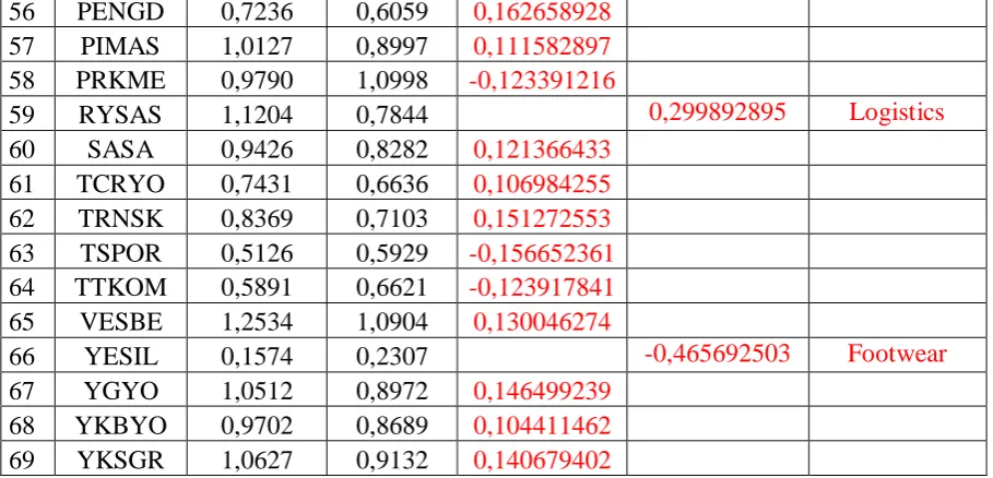
Stata 10.1 package is used to estimate the model. According to our analysis, although most of
the betas (224 of 293 securities) for the robust estimator are fairly close to the OLS beta,
considerable amount of betas (69 of 293 betas) are highly different (more than 10%) remarks.
In other words, 23,5% of the firms have differences larger than 0.1 and 6% have differences
larger than 0.2. These differences are likely to be financially significant to many investors.
Even some of the security betas have more than 20% differences. There are 69 firms that
have at least 10% different beta results, as listed in Table 1.
Table 1. Proportional Difference Between OLS and LMS Beta
FIRMS OLS BETA
LMS
BETA =10
=20 INDUSTRY
1
ADANA
A 0,9542 0,8446 0,114780167
2 AFM 0,5465 0,4722 0,136015799
3 ALYAG 0,7295 0,8319 -0,140370117
4 ANELT 0,7619 0,8491 -0,114450715
5 ANSA 0,6558 0,7893 -0,203568161 Investment B.
6 ARFYO 1,0317 0,8902 0,137152273
7 ASLAN 0,8694 0,6581 0,243041178 Cement
9 ASYAB 1,1346 1,2536 -0,104882778
10 ATAGY 0,6631 0,5876 0,113859146
11 AYCES 0,8627 0,7075 0,179900313
12 BAKAB 0,1391 0,0578 0,584471603 Packing
13 BJKAS* 1,0252 0,6676 0,348809988 Sports
14 BOYNR 1,2669 1,0788 0,14847265
15 BRMEN 0,5937 0,6655 -0,1209365
16 BOROVA 0,9831 0,7905 0,195910894
17 BRYAT 0,8968 0,7933 0,115410348
18 BSOKE -0,0321 0,0534 2,663551402 Cement
19 CCOLA 0,6095 0,6792 -0,11435603
20 CMENT 0,8132 0,5732 0,295130349 Cement
21 DAGHL 0,9927 0,8818 0,111715523
22 DENIZ 0,8298 0,6343 0,23559894 Banking
23 DEVA 0,7772 0,9171 -0,180005147
24 DGZTE 1,2576 1,0947 0,129532443
25 DNZYO 1,1243 0,7300 0,350707107 Investment B.
26 DOBUR 1,2040 1,0190 0,153654485
27 DOHOL 1,2264 1,1036 0,100130463
28 DYOBY 1,0965 0,9794 0,106794346
29 EDIP 0,8048 0,6349 0,21110835 Real Estate
30 EGPRO 0,5490 0,4250 0,225865209 Construction
31 EMKEL 0,9938 0,8332 0,161601932
32 ERSU 0,7803 0,6707 0,140458798
33 ESEMS 0,9047 0,7678 0,15132088
34 FENER 0,6466 0,4366 0,32477575 Sports
35 FFKRL 0,9757 0,8756 0,10259301
36 FINBN 0,9486 0,7631 0,195551339
37 FONFK 0,9318 0,7724 0,171066753
38 GDKGS 0,5305 0,4743 0,105937795
39 GDKYO 0,5915 0,5176 0,124936602
40 GEREL 0,9478 0,7071 0,253956531 Electrical
41 GOLTAS 0,7809 0,6702 0,141759508
42 GRNYO 1,0125 0,8356 0,174716049
43 GSRAY 0,5326 0,4255 0,201088997 Sports
44 GUBRF 0,9025 1,0363 -0,148254848
45 GUSGR 0,8223 0,9071 -0,10312538
46 HZNDR 0,7784 0,6893 0,11446557
47 ICGYH 1,1058 0,7677 0,305751492 Investment B.
48 IHLAS 1,1259 0,9455 0,160227374
49 KRDMB 1,2273 1,0805 0,119612157
50 KRSTL 1,0166 0,8105 0,202734606 Beverage
51 MEMSA 1,0701 0,9179 0,142229698
52 MRSHL 0,8527 0,7529 0,117039991
53 MZHLD 1,0150 0,8272 0,185024631
54 NUHCM 0,6479 0,5645 0,128723568
56 PENGD 0,7236 0,6059 0,162658928
57 PIMAS 1,0127 0,8997 0,111582897
58 PRKME 0,9790 1,0998 -0,123391216
59 RYSAS 1,1204 0,7844 0,299892895 Logistics
60 SASA 0,9426 0,8282 0,121366433
61 TCRYO 0,7431 0,6636 0,106984255
62 TRNSK 0,8369 0,7103 0,151272553
63 TSPOR 0,5126 0,5929 -0,156652361
64 TTKOM 0,5891 0,6621 -0,123917841
65 VESBE 1,2534 1,0904 0,130046274
66 YESIL 0,1574 0,2307 -0,465692503 Footwear
67 YGYO 1,0512 0,8972 0,146499239
68 YKBYO 0,9702 0,8689 0,104411462
69 YKSGR 1,0627 0,9132 0,140679402
Note: For all the stocks, we have regression results p<0.01 (for beta coefficient and market returns).
Another problematic issue also comes from the beta value itself. We know from the CAPM
analogy that a beta of one indicates that the securityʼs price will move with the market. A
beta less than one means that the security will be less volatile than the market. A beta greater
than 1 indicates that the securityʼs price will be more volatile than the market. However, as
seen from Table 2, two different methods might result in two distinct outcomes for the same
[image:9.595.68.523.12.231.2]stock in terms of beta movement.
Table 2. Comparison of Beta Values for Market Index Relation
FIRMS OLS BETA LMS BETA % DIFFERENCE
1 ADANA C. 1,0147 0,9617 0,052192
2 ARFYO 1,0317 0,8902 0,137152
3 BJKAS 1,0252 0,6676 0,34881
4 CELHA 1,0473 0,9679 0,075814
5 DGGYO 1,0075 0,9518 0,055285
6 DNZYO 1,1243 0,7300 0,350707
7 DYOBY 1,0965 0,9794 0,106794
8 ECZYT 0,9439 1,0153 -0,07564
9 GRNYO 1,0125 0,8356 0,174716
10 GUBRF 0,9025 1,0363 -0,14825
11 ICGYH 1,1058 0,7677 0,305751
12 IHLAS 1,1259 0,9455 0,160227
13 ISGYO 1,0018 0,9949 0,006888
14 KRSTL 1,0166 0,8105 0,202735
15 MEMSA 1,0701 0,9179 0,14223
17 MZHLD 1,0150 0,8272 0,185025
18 NTHOL 1,0390 0,9971 0,040327
19 NTTUR 1,0225 0,9805 0,041076
20 PIMAS 1,0127 0,8997 0,111583
21 PRKME 0,9790 1,0998 -0,12339
22 RYSAS 1,1204 0,7844 0,299893
23 SONME 0,9298 1,0167 -0,09346
24 USAK 1,0710 0,9896 0,076004
25 VAKFN 0,9847 1,0141 -0,02986
26 VESTL 1,0523 0,9779 0,070702
27 YATAS 1,0115 0,9775 0,033613
28 YAZIC 1,0033 0,9276 0,075451
29 YGYO 1,0512 0,8972 0,146499
30 YKSGR 1,0627 0,9132 0,140679
For example, while with the OLS regression, BJKAS beta is 1,0252, with the LMS
regression, it is calculated as 0,6676. There is a 34% difference between these two results.
Under the CAPM, when beta is greater than one, it implies that the security is more volatile
than the market index and has a chance of winning more than the market if the market index
will increase. However, while one model indicates that the BJKAS beta value is greater than
one, another indicates that it is lesser than one. It is also very difficult to decide whether the
security is more volatile than the market index or not.. Table 2 shows that 30 firms of 293
have different beta scores when OLS regression results are greater than one and LMS results
are lesser than one; and when OLS regression results are lesser than one and LMS results are
greater than one.
5. Conclusion
In our analysis, we determine two main problems when we use OLS and LMS methods for
the same data set. We compare the behavior of the OLS and LMS method beta estimates
using monthly returns (adjusted price for US dollar) for firms listed on the Istanbul Stock
Exchange (Borsa Istanbul) from the BIST 100 database. We include 293 firms that have been
listed for 150 months. Firstly, there are huge difference between OLS and LMS beta scores
69 of 293 firms. Secondly, in our analysis, OLS and LMS methods give us different beta
scores for 30 firms in terms of volatility measurement. In other word, while one method
indicates that these securities are less volatile from the market but the other method indicates
they are more volatile from the market., These results create great confusion for the many
Even only one outlier can cause these problems. Thus, We propose to use robust statistics
model for calculating beta score.
REFERENCES
Journal Papers
1. Ajlouni, Moh'd M, Dima W.H. Alrabadi Tariq K. Alnader, Forecasting the Ability of
Dynamic versus static CAPM: Evidence from Amman Stock Exchange, Jordan Journal of
Business Administration, Volume 9, No. 2. 2013
2. Zaimović, Azra, Testing The CAPM In Bosnia And Herzegovina With Continuously
Compounded Returns, South East European Journal of Economics and Business. Volume 8
(1), 31-39.
3. Cheng,Tsung-Chi, Hung-Neng Lai and Chien-Ju Lu, Industrial Effects and the
CAPM: From the Views of Robustness and Longitudinal Data Analysis, Journal of Data
Science 3(2005), 381-401, 2005.
4. Martin, R. Douglas and Tim Simin, Outlier-Resistant Estimates of Beta, Financial
Analysts Journal, Vol. 59, No. 5, 56-69, September/October, 2003.
5. Rousseeuw, Peter J., Least Median of Squares Regression, Journal of the American
Statistical Association, December, Volume 79, Number 388, Theory and Methods
Section,1984.
Thesis
1. Miao, Dingquan, Empirical Researches of the Capital Asset Pricing Model and the
Fama-French Three-factor Model on the U.S. Stock Market, Bachelor Thesis in Economics,
Division of Economics, The School of Business, Society and Engineering (EST) Mälardalens
University Västerås, 2013
Others
1. Allen, David E., Abhay Kumar Singh and Robert Powell, Asset Pricing, the
Fama-French Factor Model and the Implications of Quantile Regression Analysis, School of
Accounting, Finance and Economics & FEMARC Working Paper Series Edith Cowan
University, Working Paper 0911, October, 2009.
https://www.ecu.edu.au/__data/assets/pdf_file/0013/40432/wp0911da.pdf
2. Simonoff, Jeffrey S., CAPM: Do you want fries with that?, 2011.
http://people.stern.nyu.edu/jsimonof/classes/2301/pdf/mcdonald.pdf
3. Milionis, Alexandros E. and Dimitra K. Patsouri, A Conditional CAPM; Implications
http://www.emeraldinsight.com/doi/abs/10.1108/15265941111158488
4. Barreto, Humberto, An Introduction to Least Median of Squares, 2001
[email protected], http://www.wabash.edu/econexcel
5. Martin, R. Douglas and Tim Simin, Estimates of Small-Stock Betas are Often Very
Distorted by Outliers, Technical Report No. 351, Department of Statistics, University of
Washington, May, 1999.
https://www.stat.washington.edu/research/reports/1999/tr351.pdf
6. Jiang, Chuanliang, On the Robustness of Beta Risk In The Cross-Sectional
Regressions Of Stock Return, 2011.
https://www2.bc.edu/chuanliang-jiang/Working_Paper.pdf
7. Hodgson, Douglas J, Oliver Linton, Keith Vorkink, Testing The Capital Asset Pricing
Model Efficiently Under Elliptical Symmetry: A Semiparametric Approach, Discussion
Paper, July, 2000.
https://ideas.repec.org/p/fmg/fmgdps/dp382.html
8. Tofallis, Chris, Investment Volatility: A Critique of Standard Beta Estimation and A
Simple Way Forward, University of Hertfordshire, United Kingdom, 2014.
http://arxiv.org/ftp/arxiv/papers/1109/1109.4422.pdf
9. Genton, Marc G. and Elvezio Ronchetti, Robust Prediction of Beta, 2007.