PII. S0161171202012115 http://ijmms.hindawi.com © Hindawi Publishing Corp.
AN INTRODUCTION TO SPHERICAL ORBIT SPACES
JILL MCGOWAN and CATHERINE SEARLE
Received 21 February 2001 and in revised form 24 September 2001
Consider a compact, connected Lie groupGacting isometrically on a sphereSnof radius 1. Two-dimensional quotient spaces of the typeSn/G have been investigated extensively. This paper provides an elementary introduction, for nonspecialists, to this important field by way of several classical examples and supplies an explicit list of all the isotropy sub-groups involved in these examples.
2000 Mathematics Subject Classification: 53C20, 57S15.
1. Introduction. Spheres have long been an active area of investigation for geome-ters, algebraists, and physicists because of the richness of symmetry and beguiling simplicity they offer. In particular, a sphere is associated with an enormous group of transformations that preserve its underlying metric; these transformations are called isometries. Careful study of these actions has led to deeper understanding of spherical geometry, to the discovery of many examples of minimal submanifolds, and hypersur-faces on Stiefel manifolds and Grassmannian manifolds. Moreover, it is interesting to see how simple linear algebra reveals the secrets of the geometry of these orbit spaces. Before describing specifically the content of this paper, we present a motivating example.
Example1.1. Suppose that we allow matrices of the form
g=
cosθ −sinθ 0 sinθ cosθ 0
0 0 1
(1.1)
to operate onS2= {(x, y, z):x2+y2+z2=1}by matrix multiplication. This is a rotation around thez-axis by an angleθ. There is an obvious isomorphism between this groupG of matricesg and the circleS1= {eiθ:θ∈[0,2π )}, so we will think
x=0 x=y
Figure1.1
thexy-plane inR3, since
cosθ −sinθ 0 sinθ cosθ 0
0 0 1
x y 0 =
xcosθ−ysinθ xsinθ+ycosθ
0
. (1.2)
It also fixes the normal space, thez-axis. Because the action fixes these two normal subspaces, it is calledreducible. If we intersect the sphere with the half plane{(x,0, z): x≥0}, we have exactly one point in the sphere for each orbit. We see then that the orbit space is an interval, isometric to a closed half-circle of radius one.
Distance in the orbit space is defined to be the distance between orbits in the original space. Since the distance between the north pole and the south pole inS2isπ (half the circumference of a circle inS2joining them), this is the length of the orbit space. It is not a manifold (although it is a manifold with boundary) because of the endpoints. (SeeFigure 1.1.)
In this paper, we see how to generalize the techniques used in analyzing the ex-ample above to actions on n-dimensional spheres. We will work out several cases, as described below. In brief, the contents of this paper are as follows. InSection 2, we begin with some necessary definitions. InSection 3, we offer some background and examples from classical theory on group actions on spheres. In Section 4, we describe in detail the following reducible actions on spheres: (G, φ)= (SO(n1)× SO(n2)×SO(n3), ρn1+ρn2+ρn3), whereρnis the standard representation of SO(n),
(G, φ)=(SO(2)×SO(m), ρ2⊗ρm+1), where 1 is a one-dimensional trivial
representa-tion, and(G, φ)=(SO(k),2ρk),fork≥3. (Even though the groups in these three cases
are getting smaller, the actions are actually becoming more complicated, as we shall see. The subset of GL(n,R)for which all elementsAsatisfyA−1=AT is called O(n);
is its connected component of the identity.) InSection 5, we describe the following ir-reducible actions:(G, φ)=(SO(3)×SO(n), ρ3⊗ρn),(G, φ)=(SO(3)×SO(3), ρ3⊗ρ3), (G, φ)=(U(3)×SU(n), ρ2×µ3⊗µn), and(G, φ)=(Sp(3)×Sp(n), ν3⊗νn). InSection 6,
of concern to physicists as well as geometers. We hope this method makes this infor-mation more accessible to physicists and nonspecialists who may have an interest in these orbit spaces. Moreover, the decompositions themselves are of interest, in that many of them are not well known, especially those that correspond to irreducible actions.
Hsiang and Lawson’s classical paper on this subject [4] describes most of the orbit spaces produced by irreducible, maximal linear groups on the standard sphere and computes the principal isotropy subgroups in each case. Straume’s comprehensive work on the subject [9,10] describes not only all these actions in detail, but also actions on homotopy spheres as well. In these, he completes the proof of the classification of spheres with orbit spaces of dimensions 1 and 2. He provides the list of orbit spaces of those cases omitted by Hsiang and Lawson in [8]. Both [4,9] list the principal isotropy groups involved and, in the case of the polar actions, the associated symmetric spaces as well. The intermediate isotropy groups (i.e., those on the edges and vertices of the orbit spaces) are not explicitly included in any of these papers; however, they may be computed using the configuration of the spherical triangle in question and the list of possible cohomogeneity-one actions.
With respect to the specific examples included herein, except for the SO(3)×SO(3) example, Hsiang and Lawson [4] list all the orbit spaces resulting from the irreducible actions inSection 5 applied toRn, and their principal isotropy subgroups. In
addi-tion, they describe the orbit space resulting from the reducible SO(k)action onRn,
where the isotropy subgroups are also listed. Straume [8] also lists the orbit space resulting from this SO(k)action onS2n−1. While the orbit space resulting from the SO(3)×SO(3)action onS8can be deduced by reference to all three of [8,9,10], it is nowhere explicitly calculated. (Hsiang and Lawson [4] do include an explicit statement about the orbit spaceS8/SO(3)×SO(3), but they erroneously list it as the same orbit space asS3n−1/SO(3)×SO(n)forn >3.) The orbit spaces of the first two reducible actions inSection 4are not listed anywhere, as they are very easy to compute from the cohomogeneity-one actions, which [4,9,10] classify.
2. Definitions. In our introduction, we gave some rough definitions. Here, we will formalize some of them and add a few others. All the actions we will consider are actions on spheres which, of course, are manifolds.
Definition2.1. Ann-dimensionalmanifoldMis Hausdorff topological space
fur-nished with a collection of open setsUα, such that
(1) M=α∈AUα;
(2) on any open setUα, there is a homeomorphism,φα, fromUαtoRn, such that,
whenever the intersection of any pair of these open setsUα∩Uβis nonempty,
φα◦φβ−1|φβ(Uα∩Uβ)is a smooth (C∞) homeomorphism between subsets ofR n.
Since we restrict our attention to the standard sphereSn embedded inRn+1, for the sake of simplicity in the next definition, we assume our manifold to be embedded in Euclidean space, where we have a well-defined notion of arclength.
Definition 2.2. Thedistance d(x, y)between two pointsx and y in M is the
infimum of the lengths of all piecewise smooth curves inMthat joinxandy. This definition will satisfy all the usual properties of a metric:
(i) d(x, y)≥0, (ii) d(x, y)=d(y, x),
(iii) d(x, y)+d(y, z)≥d(x, z).
Definition2.3. Anisometry is a diffeomorphismφ:M→Nthat preserves the
distance functiondN(φ(x), φ(y))=dM(x, y).
A groupGis said to act isometrically on a manifoldMif
(i) each elementginGdefines a distance-preserving map fromMto itself, (ii) the composition of two such maps coincides with the group operationg(h(x))
=gh(x)for everyxinMand for every pairgandhinG, (iii) the identity element ofG, id, is the identity map onM.
(An example to keep in mind with respect to group actions is the group of orthog-onal matrices acting onRn.)
Definition2.4. Theorbitof a pointxis the setG(x)={y∈M:y=g(x)for some
g∈G}.
Such an action defines an equivalence relation onM, since two orbits are either identical or disjoint. (Suppose, for example,yis in the orbit ofx. Then for somegin G,g(x)=y. Then the orbit ofyis contained in the orbit ofx, sinceh(y)=h(g(x)) for everyhinG. However,g−1(g(x))=g−1(y), sox=g−1(y), andxis also in the orbit ofy. So we have containment in both directions, and the orbits must be equal.) These orbits are considered as points in a new space,M/G, called theorbit space. If M is a metric space, this orbit space is endowed with a natural metric: the distance between pointsG(x)andG(y)inM/Gis the same as the distance between the two setsG(x)and G(y)inM. WhenGis compact, this distance is zero only when the orbits coincide.
Definition2.5. In general, forMa Riemanniann-manifold, we say thatGacts by
cohomogeneitykonMwhen dim(M/G)=k.
For instance,Example 1.1exhibits a cohomogeneity-one action.
The isometries under consideration are from the sphere to itself. We will show how various orbit spaces are obtained. We will also find which subgroups ofG—called isotropy subgroups—fix different points in the manifold.
Definition2.6. When a manifold M is acted on by a groupG, the isotropy
sub-group(orstability subgroup)Gxof a pointxin the manifold is the subgroup that fixes
x; that is,Gx= {g∈G:g(x)=x}.
By the definition of a group action,Gxalways contains the identity element of the
are conjugate. Ifg(x)=y, then for anyh∈Gy,h(g(x))=h(y)=y, andg−1(hg(x))
=g−1(y)=x, sog−1hg∈G
x. Therefore,g−1Gyg⊂Gx. Sincex=g−1(y),gGxg−1⊂
Gy. Since we have containment both ways,gGxg−1=Gy. Two orbitsG(x)andG(y)
are of the same type ifGxandGyare conjugate inG.
Definition2.7. Aprincipal isotropy subgroup(in terms of dimension, the
“small-est”) is an isotropy subgroupHofGsuch that for every other isotropy subgroupK, K⊇gHg−1for someginG.
This group (all principal isotropy subgroups are conjugate and hence isomorphic) is associated with a special class of orbits.
Definition2.8. Orbits having a conjugate ofH as their isotropy subgroup are
called theprincipal orbits.
Orbits whose isotropy subgroups are of a strictly higher dimension thanH are called singular orbits.
The union of these principal orbits form an open, dense submanifold ofM, called theregular partofM[6].
InExample 1.1, the principal isotropy subgroup is the identity, because any point inS2without zero entries is not fixed by any nontrivial subgroup of the circle. That is, forxandynonzero,
xcosθ−ysinθ xsinθ+ycosθ
z
=
x y z
(2.1)
implies that cosθ=1. However, at the points(0,0,±1), the isotropy subgroup is all ofS1, because the whole circle fixes these points. Therefore, these are singular orbits, and their associated isotropy subgroup isS1.
Principal orbits form the interior of the orbit spaceM/G, and singular orbits form the boundary.
Definition2.9. Arepresentationof a groupGon a vector spaceV is
homomor-phismρ fromGto the group of all invertible linear transformations onV; that is, ρ:G→GL(V ).
A representation of Gon V is calledreducible if there is a proper, nontrivial G-invariant subspace ofV. Otherwise, it is calledirreducible.
We wish to study the representations ofG into GL(V )such thatρ(G) acts onSn
for somen. For the sake of brevity, we often writeg(v)forρ(g)(v), whenρis clear from the context.
3. Background and examples
Definition3.1. ALie group G is a group that is also a manifold, on which the
LetGbe a compact, connected Lie group, acting isometrically onSn, the standard
sphere inRn+1of radius 1.
As previously mentioned, inExample 1.1, we have an action of cohomogeneity one (since the orbit space is one dimensional). On the other hand, if we allow the entire orthogonal group to act onSn, there is only one orbit, since every pointx∈Snis the
image of the point(1,0, . . . ,0)under multiplication by a matrix with the vectorxin the first column. This is a cohomogeneity-zero action.
Definition3.2. Ageodesic on a manifoldM is a parameterized curvec whose
accelerationcis always perpendicular toM.
Example3.3. One of the classic examples of a group action on a sphere is the Hopf
actionS1acting onS3. This action can be represented as
eiθ 0
0 e−iθ
r eiα
seiβ , (3.1)
whererandsare nonnegative real numbers withr2+s2=1. This is a reducible action; it fixes the geodesicseiα
0
ande0iβ
. By choosingθ= −α, we see that a typical orbit contains a point of the type(r , seiφ); therefore, the orbit space has dimension one
less thanS3: it is two dimensional. Only the identity fixes a point of this type, so the principal isotropy group is trivial. Moreover, there are no singular orbits, and hence, no edges or vertices.
In the examples below, we find the orbit spaces and the isotropy subgroups asso-ciated with these actions through repeated use of the following facts:
(1) constant matrices, that is,kIn, wherekis a scalar, are in the center of GL(n, V ).
This is because multiplication by a scalar matrix is identical to multiplication by the scalar itself as it multiplies every entry in the other matrix by that scalar;
(2) over a commutative field such asRorC, the only matrices that commute with diagonal matrices having unequal entries along the diagonal are other diagonal matrices;
(3) the two diagonal entries in a diagonal 2×2 matrix may be interchanged through conjugation by
0 1
−1 0 . (3.2)
Consequently, any two diagonal entries in any diagonal matrix may be interchanged through an appropriate conjugation by elementary matrices.
(cf. [3, 4, 8,9,10,11]). We note that whenSn/G=D2, the singular orbits form the boundary of the disk and the singular isotropy subgroups at those points act on the unit normal subspace to the orbits by cohomogeneity one. Since the cohomogeneity-one actions have been classified, it suffices to find the singular isotropy subgroupsK withH⊂K⊂Gthat act on the normal subspace by cohomogeneity one.
Another method entails looking at the matrix representation ofGin the group of n×n orthogonal matrices O(n). We then take a “typical” vector in Sn, and try to
see howG identifies that vector with other vectors. Basically, we try to reduce the dimensions in the(n+1)-vector by replacing as many entries as possible by zero, and still remain within the same orbit. Then, we use this simplified vector to see what subgroup ofGwould fix that vector. In this way, we find the principal isotropy subgroup. We look at less typical vectors, ones with more zeros, perhaps, or more identifications among the entries, to find other possible isotropy subgroups. These computations give a very explicit description of the elements in the orbit space as subspaces inRn, and any edges and vertices. Sometimes, however, it is very difficult
to write out an explicit matrix description of the group action. Therefore, we need the two methods to complement one another.
4. Reducible examples. A whole body of very simple reducible examples is ob-tained by adding either a one-dimensional trivial action (1) or a transitive action by SO(k)to cohomogeneity-one actions on spheres. In this section, we will look at the reducible actions (G, φ)=(SO(n1)×SO(n2)×SO(n3), ρn1+ρn2+ρn3), where ρn is
the standard representation of SO(n),(G, φ)=(SO(2)×SO(m) (m >2), ρ2⊗ρm+1),
where 1 is a one-dimensional trivial representation, and (G, φ)=(SO(k),2ρk),for
k≥3. We will describe the resulting orbit spaces under these actions.
Example4.1. The action of SO(n1)×SO(n2)×SO(n3)onSn1+n2+n3−1.
If we add a transitive action by SO(n)to a cohomogeneity-one action, as in(G, φ)= (SO(n1)×SO(n2)×SO(n3), ρn1+ρn2+ρn3), we add another dimension to our orbit
space. Under this action, vectors inRn1+n2+n3are acted on by matrices of the type
A
B C
, (4.1)
whereAis in SO(n1),Bis in SO(n2), andCis in SO(n3). Each matrix may be taken to reduce the vector of the appropriate dimension to its length. Think of the appropriate vector inRn1+n2+n3 as the direct sum ofv1∈Rn1,v2∈Rn2, andv3∈Rn3; that is,
((v1), (v2), (v3)). Then, by choosing the first row in A to be a unit vector parallel
to v1, the first n1 entries of the image are reduced to (v1,0, . . . ,0). Similarly, B
and C can be chosen to reduce v2 andv3to their lengths. Thus, every orbit space
Therefore, the principal isotropy group is isomorphic to SO(n1−1)×SO(n2−1)× SO(n3−1), in a form conjugate to
1
A 1
B 1
C
, (4.2)
whereA is an element of SO(n1−1),B is an element of SO(n2−1), andC is an element of SO(n3−1). The orbit space may be described as the triangle in the two-sphere that inhabits the first octant:{(x, y, z)∈S2:x≥0; y≥0; z≥0}. The edges arex=0,y=0, and z=0. On these edges, the submatrix that corresponds to the subspace of the zero vector acts trivially, so the isotropy subgroup on the edge cor-responding to theni-dimensional vector has a factor of SO(ni)replacing the factor
SO(ni−1), SO(n1)×SO(n2−1)×SO(n3−1)is the isotropy subgroup of points for whichv1=0, for instance. At the vertices,(1,0,0),(0,1,0), and(0,0,1), two of the
SO(ni−1)factors are replaced by SO(ni). We have now found the orbit space and all
the isotropy subgroups. The decomposition of this action is given inFigure 4.1.
SO(n1)×SO(n2)×SO(n3)
SO(n1)×SO(n2)×SO(n3−1) y=0
x=0
SO(n1−1)×SO(n2)×SO(n3−1) SO(n1)×SO(n2−1)×SO(n3−1)
SO(n1)×SO(n2)×SO(n3−1) SO(n1−1)×SO(n2−1)×SO(n3−1)
z=0
SO(n1−1)×SO(n2−1)×SO(n3) SO(n1−1)×SO(n2)×SO(n3)
Figure4.1
Example4.2. The action of SO(2)×SO(m)onS2m.
Suppose, instead, that we add a trivial action to a cohomogeneity-one action. For example, take(G, φ)=(SO(2)×SO(m), ρ2⊗ρm+1). Under this action, the first 2m
entries in the(2m+1)-vector inS2mare represented as a 2×mmatrix. This matrix
is acted on by left multiplication by elements of SO(2) and by right multiplication by elements of SO(m). The last entry of the(2m+1)-vector inS2mis the object of
SO(m), respectively, can serve to “diagonalize” the 2×mmatrix, that is, to leave all the entries zero savea11anda22. (This is a standard theorem of linear algebra. See, e.g., [7, page 179].) Moreover, we may assume both entries to be positive, since either may be made positive by multiplication by an appropriate element of SO(m). As we have noted in (3), we can interchangexandy, so we may assume thatx≥y≥0. Thus, the orbit space is the subset of the two-sphere given by{(x, y, z)∈S2:x≥y≥0}. It is the spherical lune cut by the planesx=y andy =0. Along the edge x=y, the isotropy subgroup is isomorphic to SO(2)×SO(m−2), in a form conjugate to {B⊗B−1
A
:B∈SO(2); A∈SO(m−2)}.
SO(2)×SO(m)
x=y Z2×SO(m−1)
y=0
SO(2)×SO(m)
SO(2)×SO(m−2)
Figure4.2
Along the edge y = 0, the isotropy subgroup is isomorphic toZ2×SO(m−1), in a form conjugate to{±I2⊗
±1
A
:A∈O(m−1)}. (This group is also denoted S(O(1)O(m−1)).) For a fixed value ofz, the decomposition of the orbit space is exactly the same as it is for the cohomogeneity-one action. Thus, the decomposi-tion of the cohomogeneity-two acdecomposi-tion may be thought of as a suspension of the cohomogeneity-one action along each levelz=cbetween the poles. The poles,z= ±1, are fixed points under the action. InFigure 4.2, there is a diagram of the orbit space and the isotropy decomposition for the cohomogeneity-two action.
Example4.3. The action of(G, φ)=(SO(k),2ρk)onS2k−1.
Finally, we examine a reducible cohomogeneity-two action that is not a direct sum with a cohomogeneity-one action:(G, φ)=(SO(k),2ρk),fork≥3. Under this action,
SO(k)acts onR2kby matrices of the form
A
A , (4.3)
whereAis in SO(k). We can think of the firstkentries of the vector inR2kas one
vector, v1, inRk, and the second kentries as another, v2. If these two vectors are
SO(k)
SO(k−2)
SO(k−1)
Figure4.3
ofk-vectors, the image of theR2kvector under multiplication by this matrix will be
a vector of the form(x,0, . . . ,0;y, z,0, . . . ,0), withx≥0, andz≥0. (The semicolon signifies the end of the firstk-vector.) The principal isotropy subgroup will therefore be a conjugate of the group of matrices of the form
I2
B I2
B
, (4.4)
whereBis in SO(k−2). We have larger isotropy subgroups when rank(v1,v2)=1.
Then, either v1 is parallel tov2 or one of the vectors is zero. If they are parallel,
the orbit has an element of the form (x,0, . . . ,0;y,0, . . . ,0), and the isotropy sub-group is isomorphic to SO(k−1). The isotropy subgroup is also SO(k−1)if either v1=0orv2=0, because the orbit representative is the same, except that eitherx
or y is zero. The orbit space is therefore a disk without vertices. In fact, it is the upper hemisphere of the sphere of radius 1/2. We can see this by inspecting the geodesics of the orbit space. The boundary geodesic is(cosθ,0, . . . ,0; sinθ,0, . . . ,0). This geodesic closes at θ = π, since x =1 and x = −1 are identified; it reaches its most distant position atθ =π /2. Longitudinal geodesics may be described as (cosαsinφ,0, . . . ,0; sinαsinφ,cosφ,0, . . . ,0), where α ∈ [0, π ) is fixed, and φ ∈ [−π /2, π /2). As mentioned above,(x,0, . . . ,0;y,0, . . . ,0)and(−x,0, . . . ,0;−y,0, . . . ,0) are identified under the group action, so the geodesic closes there. The piece of the ge-odesic that lies in the orbit space is that with cosφ >0. This is half the geodesic; it has lengthπ /2. These geodesics are perpendicular to the underlying orbits, because no element of the group action changes the lengths ofv1orv2, and the geodesic moves
strictly in the direction that would change these lengths. The restrictionz≥0 makes this orbit space the upper hemisphere. The orbit space diagram is given inFigure 4.3. The resulting orbit spaces for the reducible cohomogeneity-two actions onSnabove
are given inTable 4.1.
Here, we label a spherical lune with both anglesπ /n asDn, a spherical triangle
Table4.1
Group Representation Orbit space
SO(n1)×SO(n2)×SO(n3) ρn1+ρn2+ρn3 ∆2,2,2
SO(2)×SO(m) ρ2⊗ρm+1 D4
SO(k) 2ρk (1/2)S2(1/2)
x=0 x=yy=z
K3 α3 L1
H L2 α1 α2
L3 K1 K2
Figure4.4
Table4.2. Reducible cohomogeneity-two orbit spaces.
Group SO(n1)×SO(n2)×SO(n3)
Representation ρn1+ρn2+ρn3
Angles α1=π /2,α2=π /2,α3=π /2 H SO(n1−1)×SO(n2−1)×SO(n3−1) L1 SO(n1−1)×SO(n2−1)×SO(n3) L2 SO(n1)×SO(n2−1)×SO(n3−1) L3 SO(n1−1)×SO(n2)×SO(n3−1) K1 SO(n1−1)×SO(n2)×SO(n3) K2 SO(n1)×SO(n2−1)×SO(n3) K3 SO(n1)×SO(n2)×SO(n3−1)
Group SO(2)×SO(m) SO(k)
Representation ρ2⊗ρm+1 2ρk
Angles α1=π /4,α2=π /4,α3=π α1=π,α2=π,α3=π H Z2×SO(m−2) SO(k−2)
L1 Z2×SO(m−1) SO(k−1) L2 SO(2)×SO(m−2) —
L3 — —
K1 SO(2)×SO(m) — K2 SO(2)×SO(m) —
hemisphere of the sphere of radiusras(1/2)S2(r ). The third orbit space is computed and described in both [4, 8]; the other two may be readily seen by reference to the cohomogeneity-one actions described in [4,9,10].
Moreover, they have decompositions as given inTable 4.2, whereH,Li, andKiare
the isotropy subgroups associated with the orbit space as inFigure 4.4. The principal isotropy groups here are also presented in [4, 9,10]. The others may be computed easily with reference to [9,10].
5. Irreducible examples. In this section, we will examine the following irreducible actions:(G, φ)=(SO(3)×SO(n), ρ3⊗ρn)onS3n−1,(G, φ)=(SO(3)×SO(3), ρ3⊗ρ3)on S8,(G, φ)=(U(3)×SU(n), ρ
2×µ3⊗µn)onS6n−1, and(G, φ)=(Sp(3)×Sp(n), ν3⊗νn)
onS12n−1. Each of these examples relies on the following fact from linear algebra: an arbitrary real (complex, quaternion)n×mmatrix may be “diagonalized” under left multiplication by ann×n orthogonal (unitary, symplectic) matrix and right multi-plication by anm×morthogonal (unitary, symplectic) matrix. By “diagonalized,” we mean that the only nonzero terms are among the entriesaii. (See [7, page 179].) All
four of the following group actions result in spherical triangles as orbit spaces, so rather than include a figure for each one, we have included one figure at the end of the section to describe them all.
Example5.1. The action of SO(3)×SO(n),n >3, onS3n−1.
One action that generates a triangular orbit space is(G, φ)=(SO(3)×SO(n), ρ3⊗ ρn), wheren >3. Under this action, points ofS3n−1are represented as 3×nmatrices,
operated on by SO(3)under left multiplication, and by SO(n)by right multiplication. Appropriate choices for the left and right multipliers will reduce the middle matrix (X) to one of the form
a 0 0 0 ··· 0 b 0 0 ··· 0 0 c 0 ···
, (5.1)
wherea2,b2, andc2are eigenvalues ofXXT.
These matrix actions render the signs ofa,b, andcimmaterial and allow for shifts in the order of these entries so thata≥b≥c≥0. Sincea2,b2, andc2are eigenvalues ofXXT, no further identifications are possible. The orbit space is therefore the
spher-ical triangle{(x, y, z)∈S2:x≥y≥z≥0}. Since a diagonal matrix is fixed under conjugation by other diagonal matrices, the principal isotropy group is conjugate to
A⊗
A−1 0
0 B
, A∈SO(3), Aa diagonal matrix, B∈O(n−3)
. (5.2)
On one edge of the spherical triangle, wherez=0, the points will be fixed under multiplication by group elements of the form
A 0
0 ±1 ⊗
A−1 0
0 B
, A∈O(2), Aa diagonal matrix, B∈O(n−2)
. (5.3)
That is, the upper block matrix, which conjugates the nonzero entries inX, can be shrunk to a 2×2 block, since thezentry is now zero. The isotropy subgroup is there-foreS(O(1)O(1)O(n−2)).
On the edges where x=y or y =z, the 2×2 constant matrix is preserved by conjugation by block matrices in O(2). The third (unequal) entry can still be con-jugated by −1. The isotropy subgroup on these edges is therefore isomorphic to S(O(2)O(1)O(n−3)).
The orbit space, which is a spherical triangle, has anglesπ /2,π /3, andπ /4. The isotropy subgroup aty=z=0 is isomorphic toZ2×SO(2)×SO(n−1), since the zero-block matrix will be unaffected by any matrix multiplication. The isotropy subgroup at the intersection ofx=yand z=0 is isomorphic to SO(2)×Z2×SO(n−2), in a form conjugate to
A 0
0 ±1 ⊗
A−1 0
0 B
, A∈O(2), B∈O(n−2)
, (5.4)
since the 2×2 block matrix with equal entries on the diagonal will commute with any 2×2 matrix. At the point wherex=y=z, the isotropy subgroup is isomorphic to S(O(3)O(n−3)), since at this vertex, the 3×3 scalar block of the matrixX is fixed under conjugation by any element of O(3).
Example5.2. The action of SO(3)×SO(3)onS8.
A related action, but with a different orbit space,(G, φ)=(SO(3)×SO(3), ρ3⊗ρ3), can again reduce the spherical 3×3 matrix (X) to diagonal form, where the squares of the diagonal entries are the eigenvalues ofXXT. As before, we can interchange any
pair of these entries. However, we can no longer change the sign of a single entry, but must change them two at a time, since we no longer have the freedom to insert a−1 entry below the upper 3×3 matrix in the right factor. Thus, we can ensure only that the entries are in order of descending absolute value and that the first two are positive:{(x, y, z)∈S2:x≥y≥ |z|}. This triangle is the double of the triangle under the SO(3)×SO(n)action, reflected through the planez=0. The edges of this triangle are the intersections of the two-sphere with the planesx=y,y=z, andy= −z.
isotropy subgroups on these two edges areS(O(2)O(1))and S(O(1)O(2)), respec-tively. Moreover, we get an isomorphic group on the edgey= −z
±1
A I2
−1
x 0 0
0 y 0
0 0 −y ±1
A−1 I2
−1
, (5.5)
whereA∈SO(2)if the±1 in the upper-right corner is negative, andA∈O(2)with determinant−1, if the sign of the 1 is positive. (Thus, the product of the first two factors is in SO(3).) The isotropy subgroups on the vertices are computed analogously with those in the previous action, except in the case of the third vertex, where we again multiply on both sides byI2
−1
to make the most use of the symmetries.
Example5.3. The action of U(3)×SU(n)onS6n−1.
We can apply a similar action with the unitary group(G, φ)=(U(3)×SU(n), (ρ2× µ3)⊗µn). The unitary group action behaves very similarly to the real action: the left
and right multiplication can reduce the 3×nmatrixXto the three nonzero entries
x 0 0 0 ···
0 y 0 0 ···
0 0 z 0 ···
. (5.6)
The squares of these entries are the eigenvalues ofXXT, which are real becauseXXT is Hermitian. Therefore, the entriesx,y, andzare either real or purely imaginary; they can be made real by multiplication by an appropriate element of U(3). They can be arranged in order of descending absolute value, and, because the first factor group is U(3), they can all be made positive; the orbit space is
(x, y, z)∈S2:x≥y≥z≥0. (5.7)
The principal isotropy subgroup isS(U(1)3U(n−3)), as any of the entries,x,y, or z, can be conjugated by eiθ. On the edges and vertices, the isotropy subgroups are
analogous to those under the SO(3)×SO(n)action.
Example5.4. The action of Sp(3)×Sp(n)onS12n−1.
The action by the symplectic group(G, φ)=(Sp(3)×Sp(n), ν3⊗νn), where Sp(n)
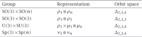
Table5.1
Group Representation Orbit space
SO(3)×SO(n) ρ3⊗ρn ∆2,3,4 SO(3)×SO(3) ρ3⊗ρ3 ∆2,3,3 U(3)×SU(3) ρ2×µ3⊗µn ∆2,3,4 Sp(3)×Sp(n) ν3⊗νn ∆2,3,4
we use the unitary matrix that would diagonalizeXTX, which is a 2n×2ncomplex matrix of the formA−B
B A
. For any matrix of this form, if((u), (v))is an eigenvector with eigenvalue λ, then((−v), (u))is also an eigenvector, with eigenvalue λ. Since the unitary matrix that diagonalizesXTXby conjugation has the eigenvectors ofXTX as its columns, it, too, can be written in the desired form. Therefore, there exists a 2n×2nunitary matrixU2of the desired form that diagonalizesX
T
X.
U2X T
XU2−1=
β1 0 ··· 0 0 β2 ··· 0
. ..
0 ··· 0 β2n
. (5.8)
The diagonal entries in the resulting matrix (βi) are the eigenvalues of X T
X; they are therefore real and nonnegative. If the column vectors ofXU−1
2 arev1,v2, . . . ,v2n,
equation (5.8) shows thatvi,vj =βiδij. At least 2n−6 of the βi are zero. Since
the eigenvalues ofXTXcome inλ,λpairs, there is an even number of zeros. Since XandU2are both in the subgroup of complex matrices that represent quaternionic matrices, their product is, so the zeros are evenly distributed in the upper and lower matrices. Therefore, forβinonzero, thevi/
βiform an orthonormal system, and we
can letU1be a unitary matrix withvTi/
βias itsith row for each nonzeroβ. Then
U1XU2−1is a diagonal matrix, andU1and U2are symplectic matrices. The diagonal entries areλ1,λ2,andλ3and their conjugates. Since theλiare real, they are equal to
their conjugates. We may assume that they are positive and arranged in descending order. Therefore, the orbit space is
(x, y, z)∈S2:x≥y≥z≥0. (5.9)
The isotropy subgroups may be more easily determined by reference to the quater-nionic form of the matrices if we remember that the center of the quaterquater-nionic group is the reals. Then the reasoning runs analogously to that for U(3)×SU(n).
Therefore, we see that the resulting orbit spaces for these four irreducible cohomo-geneity-two actions onSnare given inTable 5.1.
Moreover, they have decompositions as given in the following table, whereH,Li,
andKiare the isotropy subgroups associated with the orbit space as in the following
[image:15.498.125.374.97.162.2]x=0 x=yy=z
K3 α3 L1
H L2 α1 α2
L3 K1 K2
Figure5.1
Table5.2. Irreducible cohomogeneity-two actions.
Group SO(3)×SO(3) SO(3)×SO(3)
Representation ρ3⊗ρn ρ3⊗ρ3
Angles α1=π /2,α2=π /4,α3=π /3 α1=π /3,α2=π /2,α3=π /3 H S(O(1)2×O(n−3)) S(O(1)3)
L1 S(O(1)×O(2)×O(n−3)) S(O(1)×O(2)) L2 S(O(2)×O(1)×O(n−3)) S(O(2)×O(1)) L3 S(O(1)2×O(n−2)) S(O(1)×O(2)) K1 S(O(2)×O(n−2)) SO(3)
K2 S(O(1)×O(n−1)) S(O(2)2) K3 S(O(3)×O(n−3)) SO(3)
Group U(n)×SU(n) Sp(1)×Sp(n)
Representation ρ3⊗µ3⊗µn ν1⊗νn
Angles α1=π /2,α2=π /4,α3=π /3 α1=π /2,α2=π /4,α3=π /3 H S(U(1)3×U(n−3)) Sp(1)3×Sp(n−3)
L1 S(U(1)×U(2)×U(n−3)) Sp(1)×Sp(2)×Sp(n−3) L2 S(U(2)×U(1)×U(n−3)) Sp(2)×Sp(1)×Sp(n−3) L3 S(U(1)2×U(n−2)) Sp(1)2×Sp(n−2) K1 S(U(2)×U(n−2)) Sp(2)×Sp(n−2) K2 S(U(1)×U(n−1)) Sp(1)×Sp(n−1) K3 S(U(3)×U(n−3)) Sp(3)×Sp(n−3)
6. Conclusions. Much has been written about isometric actions on spheres, and in particular, cohomogeneity-two actions have been studied by a great number of people. Here, we have tried to give accessible, explicit descriptions of how these orbit spaces and their underlying isotropy groups are computed.
disks may have zero, one, two, or three vertices. The angles at these vertices may be π /2,π /3,π /4,orπ /6. In the case of irreducible actions, the orbit spaces are limited to the spherical triangles∆2,3,4,∆2,3,3, and∆2,2,3. These are all subsets of the two-sphere of radius 1 or 1/2.
Some questions that remain in this area include:
(1) what are the orbit spaces associated with actions of cohomogeneity two on manifolds of strictly positive sectional curvature? It is well known [1] that these orbit spaces will be two-spheres or disks and we know geometrically that any such disk can have at most three vertices, so the question remains as to which angle configurations occur; and similarly,
(2) what are the orbit spaces associated with cohomogeneity-three actions on spheres (and on manifolds of strictly positive curvature)? In particular, the ac-tions themselves are yet to be classified.
Acknowledgment. This work was supported in part by Consejo Nacional de
Ciencia y Tecnologia, CONACYT project number 28491-E.
References
[1] G. E. Bredon,Introduction to Compact Transformation Groups, Pure and Applied Mathe-matics, vol. 46, Academic Press, New York, 1972.
[2] R. Gilmore,Lie Groups, Lie Algebras, and Some of Their Applications, John Wiley & Sons, New York, 1974.
[3] K. Grove and S. Halperin,Dupin hypersurfaces, group actions and the double mapping cylinder, J. Differential Geom.26(1987), no. 3, 429–459.
[4] W.-Y. Hsiang and H. B. Lawson Jr.,Minimal submanifolds of low cohomogeneity, J. Differ-ential Geometry5(1971), 1–38.
[5] W. Klingenberg, A Course in Differential Geometry, Graduate Texts in Mathematics, vol. 51, Springer-Verlag, New York, 1983.
[6] D. Montgomery, H. Samelson, and C. T. Yang,Exceptional orbits of highest dimension, Ann. of Math. (2)64(1956), 131–141.
[7] I. Satake,Linear Algebra, Pure and Applied Mathematics, vol. 29, Marcel Dekker, New York, 1975.
[8] E. Straume,On the invariant theory and geometry of compact linear groups of cohomo-geneity≤3, Differential Geom. Appl.4(1994), no. 1, 1–23.
[9] ,Compact connected Lie transformation groups on spheres with low cohomogeneity. I, Mem. Amer. Math. Soc.119(1996), no. 569, vi+93.
[10] ,Compact connected Lie transformation groups on spheres with low cohomogeneity. II, Mem. Amer. Math. Soc.125(1997), no. 595, viii+76.
[11] F. Uchida,An orthogonal transformation group of(8k−1)-sphere, J. Differential Geom. 15(1980), no. 4, 569–574.
Jill McGowan: Department of Mathematics, Howard University, Washington, DC
20059, USA
E-mail address:[email protected]
Catherine Searle: Instituto de Mathemáticas de la UNAM, Unidad Cuernavaca,
Avenida Universidad S/N, Colonia lo Mas de Chamilpa, Cuernavaca, Morelos62210, Mexico