2019 International Conference on Artificial Intelligence and Computing Science (ICAICS 2019) ISBN: 978-1-60595-615-2
River Flow Forecasting Using Long Short-term Memory
Demba COUTA, Yi-kui ZHANG
and You-meng LI
*College of Intelligence and Computing, Tianjin University, China
*Corresponding author
Keywords: Flow forecasting, LSTM, Neural networks, Hyperparameters optimization, GWLF.
Abstract. In this paper we propose an LSTM application to hydrological problem, the flow estimation in Jinhe river in China. The LSTM is a very powerful prediction tool that considers temporal dependencies. The model's performance highly depends on the so-called hyperparameters values. To find the best combination of hyperparameters we have used the random search method, that is, testing combinations of randomized hyperparameters until we get the best one. We then compare the built model with a watershed model called GWLF. Using two performances indicators that are the RMSE and Nash coefficient, we found that our model is much better in both calibration and validation period.
Introduction
Many flow estimation models have been proposed for several centuries in that they allow, inter alia, agricultural water management, flood and water shortages avoidance [1-3]. The first one was established by Perreault (1674) on the Seine watershed in Paris. According to him the flow was one-sixth of the rain [4]. Since then, several models have emerged. The most natural approach in establishing a model is to try to find mathematical relationships between the different physical phenomena that cause the flow and the flow itself. These physically based models have been extensively developed over the past centuries. These models have the advantage of being applicable on several locations, but they are complex and slow. To overcome this, Conceptual models are used. These are models that use calibration in addition to the field data integrating simplified physical laws [5, 6]. The implementation of these models requires a good understanding of the hydrologic process. But in many cases, it is more optimal to use models that does not demand that comprehension. In such situations, “BLACK BOX” models are preferred. They attempt to establish a direct relationship between the input and output data without really considering hydrological mechanisms[5, 7]. They have the particularity to apply only on a specific domain [6, 7]. When we change location, for example, we often need to rebuild the model. But they have speed and usually perform well.
Artificial neural networks are one of the most used “black-box” models which can be used in many scientific and technological areas. They were presented for the first time in 1943 by W. McCulloch and W. Pitts who showed that they can perform complex logical, arithmetic and symbolic functions. But it was not until the 90s that they became an interesting subject thanks to deep learning and to the computing power of the GPUs.
Since the flow estimation is related to the concept of time, it may be wise to use recurrent neural networks (RNN), as it can process temporal data.
In this article, we propose an LSTM (Long Short-Term Memory) model, which is a particular RNN, to forecast the flow of the Jinghe River. Then we will compare it to a model called GWLF. But before that, we will give a brief overview of these two concepts.
Long Short-Term Memory (LSTM)
Long Short-Term Memory are an extension of RNN which also is an extension of ANN. So, let’s first see what ANN and RNN are.
respectively and the others are the hidden layers. Artificial neurons are elementary units in the network. An artificial neuron receives one or more inputs and produce an output.
Neural networks work by adjusting the weights (for each batch) in order to minimize the inconsistency between predicting values and real values. That inconsistency is calculated by the so-called loss function or cost function.
The essential difference between RNN and traditional neural networks is the temporal dependences. In fact, RNN use for each training example information from previous one. The applied backpropagation is called backpropagation through time, unless forward pass backward pass is entirely linear. So, if we have large dataset, the gradient tends to:
-decrease exponentially preventing the model from learning (updated parameters approximately equal to old parameters): it’s the vanishing gradient problem[9].
-increase exponentially causing instability of the model or even overflow parameter: it’s the exploding gradient problem.
To fix those issues, one of the most effective solutions is to use Long Short-Term Memory (LSTM). Proposed by Sepp Hochreiter and Jürgen Schmidhuber, LSTM models are mainly designed to avoid vanishing gradient problem. To do so a cell, an input gate, an output gate and a forget gate have been added for each unit. The cell stocks the information while the three gates regulate it.
= ( ∗ + ∗ + (1)
= ( ∗ + ∗ + ) (2)
ĉ = tanh( ∗ + ∗ + ) (3)
= ∗ + ∗ ĉ (4)
= ( ∗ + ∗ + !) (5)
H# = o# ∗ tanh(c#) (6)
where indicates forget gate, input gate, output gate and the cell state.
Generalized Watershed Loading Function (GWLF)
The GWLF is a simpler, continuous process-based model, which can estimate monthly streamflow, monthly watershed erosion and sediment yield, monthly total nitrogen and phosphorus loads in streamflow, annual erosion from each land use etc. In this study we will only focus on the monthly streamflow. Compared to other watershed models like SWAT, GWLF is relatively user-friendly as it has less needed space data, fewer parameters, relatively simplified mechanism and so on[10].
Case Study
In this study, data were collected from Jinghe river. The latter is a tributary of the Yellow River located in the central Loess Plateau and crosses three provinces (Ningxia, Shaanxi and Gansu). it covers 45,421 km²[11]. It lies between 105 490-108 580E and 34 140- 38 100N, and an average elevation about 1,200 m above sea level[12].
These collected data are daily average temperature, maximum temperature, minimum temperature, precipitation, small evaporation, sunshine hours and the corresponding flow rate from 1974/01/01 to 1987/12/31. Data from 1974/01/01 to 1982/12/31 were chosen as training set and data from 1983/01/01 to 1987/12/31 were chosen as test set.
Modeling
First, to get all data on the same scale and facilitate the learning, data are normalized to range [0, 1]; each value x replaced by x’ such that
&'= ( ) * (()
Forecasting with LSTM requires non-easy choices about the hyperparameters: timestep, batch size, epochs, number of layers, number of units for each layer. The traditional method to find the best hyperparameters is grid search, also called parameter sweep. It is a question of exhaustive searching through a subset of possible manually defined hyperparameters the combination which makes it possible to obtain the best performance. one of its advantages is that the treatments can be parallelized because they do not depend on each other. By cons it is a computationally expensive approach in our case because we'll need to evaluate more than one million combinations to optimize all the 6 hyperparameters even if we choose fairly small and manually selected sets for each hyperparameter. We then choose an alternative approach: the randomized search method. The latter is much less computationally expensive and is also embarrassingly parallel. it is a question of using random combinations to find the one which provide the best performance for the built model.
[image:3.612.141.473.234.390.2]The procedure used to find the best combination of hyperparameters is shown by figure 1.
Figure 1. Algorithm to find the best hyperparameters.
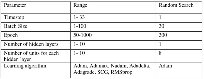
[image:3.612.131.482.457.593.2]Each hyperparameters is randomized in a manually defined range. The tested ranges and the value obtained by the random search method for each hyperparameters are shown in table 1.
Table 1. Hyperparameter tuning using random search.
Parameter Range Random Search
Timestep 1- 33 1
Batch Size 1-100 30
Epoch 50-1000 300
Number of hidden layers 1- 10 1
Number of units for each hidden layer
1- 10 8
Learning algorithm Adam, Adamax, Nadam, Adadelta, Adagrade, SCG, RMSprop
Adam
As the GWLF works with monthly values, we have converted the daily observed and LSTM forecasted flow values to total monthly flow values in order to be able to compare the performances.
Result and Discussion
Figure 2a, 2b and Figure 3a, 3b show the matching between Observed flows and the two models forecasted ones in calibration and validation period, respectively. While figure 2c and figure 3c show errors between observed and forecasted flows calculated by the following formula error=|forecasted - observed|. We can notice that:
flows except the peaks like the maximum flow rate which is the worse and was predicted as 1146.089111m/s while the real value is 1408.500122, an underestimation of 18.63%. Apart from peaks there is no underestimation which exceed 7% and no overestimation.
- The LSTM model also gives much better match in validation period. Like in the calibration period the peaks match less but this time the maximum underestimation is 13.60 % for the LSTM model while there is a maximum underestimation of 32.23% and a maximum overestimation of 44.14% for the GWLF.
Note that there is no overestimation for the LSTM model.
According to these previous figures the LSTM model performs better than the GWLF. These plots are backed with statistical performance in table 2.
a. Observed and LSTM modeled flows 1974-1982 b. Observed and GWLF modeled flows 1974-1982
[image:4.612.88.519.199.429.2]c. error between target and predicted 1974-1982
Figure 2. Comparison between LSTM and GWLF model from January 1974 to December 1982 (calibration period).
a. Observed and LSTM modeled flows 1983-1987 b. Observed and GWLF modeled flows 1983-1987
c. error between target and predicted 1983-1987
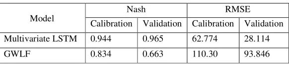
[image:4.612.91.520.476.583.2]Table 2. Models’ performances.
Model
Nash RMSE
Calibration Validation Calibration Validation
Multivariate LSTM 0.944 0.965 62.774 28.114
GWLF 0.834 0.663 110.30 93.846
The Nash–Sutcliffe model efficiency coefficient is mostly used for hydrological models and is calculated by the following formula.
NSE = 1 −∑ (23 43)²6789
∑ (43 :̅)²6
789 (8)
where x̅ is the mean of observed discharges, Yi and Xi are modeled and observed discharge at
iteration i, respectively.
It is always in range from −∞ to 1. Higher value is better than lower one, thus the perfect one is achieved at 1. In our case the Multivariate LSTM model gives greater Nash coefficient,0.944 in calibration period and 0.965 in validation period, while the GWLF model gives 0.834 in calibration period and 0.663 in validation period as Nash coefficient.
Root Mean Square Error (RMSE) is given by the following formula:
<=>? = @*∑ ( − &̅)²*
A! (9)
The RMSE is always positive and the optimal value is 0. With the same data, the model which has lower RMSE performs better. In our case RMSE of the Multivariate LSTM model provides lower RMSE which is 62.774 in calibration period and 28.114 in validation period while the GWLF provides 110.30 in calibration period and 93.846 in validation period.
Conclusion
A multivariate LSTM forecasting model has been developed and compared to the GWLF to estimate the Jinghe river flow rate. According to the RMSE and Nash coefficient, our forecasting model is better than the GWLF one in both calibration and validation period. The main difficulty was finding the right parameters like timestep, batch size, epochs, number of layers, number of units for each layer, and so on. By using the random search method we have overcome. To go further one could try to add more weather data like wind speed to the LSTM model or try to use a univariate model to evaluate the impact of the weather input.
References
[1] Ö. KİŞİ, “Daily river flow forecasting using artificial neural networks and auto-regressive models,” Turkish Journal of Engineering and Environmental Sciences, vol. 29, no. 1, pp. 9-20, 2005.
[2] D. Lekkas and C. Onof, “Improved flow forecasting using artificial neural networks,” in
Proceedings of the 9th International Conference on Environmental Science and Technology, Rhodes island, Greece, 2005, pp. 1-3.
[3] T. Partal, “River flow forecasting using different artificial neural network algorithms and wavelet transform,” Canadian Journal of Civil Engineering, vol. 36, no. 1, pp. 26-38, 2008.
[4] N. Chkir, “Mise au point d'un modèle hydrologique conceptuel intégrant l'état hydrique du sol dans la modélisation pluie-débit,” Ecole Nationale des Ponts et Chaussées, 1994.
[6] G.K. Devia, B. Ganasri, and G. Dwarakish, “A review on hydrological models,” Aquatic Procedia, vol. 4, pp. 1001-1007, 2015.
[7] Y.B. Dibike and D.P. Solomatine, “River flow forecasting using artificial neural networks,”
Physics and Chemistry of the Earth: B: Hydrology, Oceans and Atmosphere, vol. 26, no. 1, pp. 1-7, 2001.
[8] N. Karunanithi, W.J. Grenney, D. Whitley, and K. Bovee, “Neural networks for river flow prediction,” Journal of computing in civil engineering, vol. 8, no. 2, pp. 201-220, 1994.
[9] S. Hochreiter, Y. Bengio, P. Frasconi, and J. Schmidhuber, “Gradient flow in recurrent nets: the difficulty of learning long-term dependencies,” ed: A field guide to dynamical recurrent neural networks. IEEE Press, 2001.
[10]Z. Qi, G. Kang, C. Chu, Y. Qiu, Z. Xu, and Y. Wang, “Comparison of SWAT and GWLF Model Simulation Performance in Humid South and Semi-Arid North of China,” Water, vol. 9, no. 8, p. 567, 2017.
[11]G.Y. Qiu, J. Yin, F. Tian, and S. Geng, “Effects of the “Conversion of Cropland to Forest and Grassland Program” on the water budget of the Jinghe River catchment in China,” Journal of Environmental Quality, vol. 40, no. 6, pp. 1745-1755, 2011.