Neural Network for Mapping Full Time Apparent Resistivity Solution from TEM Electromotive Force Data

2018 International Conference on Physics, Computing and Mathematical Modeling (PCMM 2018) ISBN: 978-1-60595-549-0

Neural Network for Mapping Full Time Apparent Resistivity Solution from

TEM Electromotive Force Data

Ming-hui BAO

, Shan-qiang QIN

*, Guo-jun HE

, Jun-qiang Li

and Zhi-hong FU

1_{Electric Power Research Institute, Chongqing Electric Power Company Chongqing, China}

2_{Department of Electrical Engineering Theory and New Technology, School of Electrical}

Engineering, Chongqing University, Chongqing, China

3_{Chongqing Triloop Prospecting Technology Co., Ltd, Chongqing, China}

*Corresponding author

Keywords: Transient electromagnetic, Full time apparent Resistivity, Central loop, Apparent resistivity, Neural networks, Backpropagation.

Abstract. The apparent resistivity of the induced electromotive force observed by the transient electromagnetic (TEM) in center loop is proposed by using the neural network. According to the characteristics of increasing of the induced electromotive force with the resistivity of the transient electromagnetic sounding, the neural network input and output relationship and the network structure of the transient electromagnetic induction electromotive force response are designed according to the uniform half space central line observation mode. The nonlinear model of transient electromagnetic induction electromotive force and apparent resistivity is fitted by the neural network to obtain the full apparent resistivity value of the measured induced electromotive force data at a certain sampling time, and the aim of resistivity and imaging is achieved quickly. Through the calculation and verification of the simulation model of the transient electromagnetic in grounding grids, the apparent resistivity section can be obtained, and the position of the breakpoint can be clearly determined, and the effect of solving the inverse problem is achieved. The calculation of the verification model shows that the method makes the calculation time of the transient electromagnetic apparent resistivity greatly shorten, which is a practical algorithm.

Introduction

The transient electromagnetic method is a geophysical detection method based on sending the rapid turn-off of step impulse current and picking up the secondary electromagnetic field after the step impulse current turning off to detect the resistivity distribution and buried depth of target. Apparent resistivity is a parameter used to reflect the conductivity distribution in the detection area. Apparent resistivity is a widely used parameter in TEM imaging [1-3]. Analytical expression of apparent resistivity was developed in the 1980s [1]. The response of terrestrial three-dimensional (3-D) models is complex and computationally expensive, so many scholars have developed methods of rapid apparent resistivity solution.

The apparent resistivity of the central-loop TEM is calculated from the analytical expression or using the finite series expansion and an iterative algorithm for fitting the curve between the observed data and the theoretical data [1-3]. A single value of the all-time apparent resistivity is obtained for the vertical component 𝐵_𝑧 of magnetic field and Newton's dichotomy or Newton's iterative method is usually used to iteratively solve the nonlinear equations of the secondary field and various TEM parameters to calculate the expected result [4]. Bai et al. give a numerical calculation method for the time-domain transient electromagnetic apparent resistivity according to the characteristic of the kernel function for 𝜕𝐵𝑧⁄𝜕𝑡[10]. The all-time apparent resistivity iteration inverse method was

Algorithm to compute all-time resistivity rapidly and accurately based on [9]. Fu et al. proposed a method of calculating the all-time apparent resistivity using the turn-off time as one of the system parameters [5,7,14]. The algorithm for solving apparent resistivity of these scholars has its own characteristics, but there are some problems such as complex computations, early stage or late stage segmentation and initial value iteration, and there are no advantages in real-time. In the case of multi survey lines and high density measurement points, it often consumes considerable computing resources and time, and that cannot achieve the purpose of real-time rapid imaging.

Back-propagation neural network is an effective neural network, the mean square error function of back propagation algorithm exists and is differentiable. The use of neural networks in geophysical prospecting is also very popular. Neural network is a universal approximator, which approximates the arbitrary accuracy of any continuous function [6]. The neural network is used to map the transient field parameter values corresponding to the kernel function variables related to the measured data to fit the secondary eddy current curve and avoid the calculation of specific complex electromagnetic fields or numerical inverse problems to achieve the objective of solving inverse problems rapidly [14].

In this paper, a new method for directly mapping apparent resistivity of the measured EMF data each measurement point is proposed using the neural network of each time window to map of each measuring point from the earliest sampling window to the latest sampling window. According to the characteristic that the induced electromotive force decreases monotonously with the increase of resistivity, we mapped the apparent resistivity values corresponding to the measured electromotive force data measured at a certain sampling time point through fitting the induced electromotive force curve using the built neural network, and the parameter for geological information called as resistivity (conductivity) was obtained by calculation observed data.

Transient Electromagnetic Apparent Resistivity Solution Using ANN

Apparent Resistivity Solution of TEM

Transmitter of the central-loop TEM sends the step impulse current by a horizontal loop on surface of the ground. The spatial distribution characteristics of resistivity are obtained by solving the inverse problem. The transient electromagnetic response of induced electromotive force 𝜕𝐵_𝑧⁄𝜕𝑡 on the center of transmitter loop in a uniform half-space can be expressed as [1]





2 0

3

2

( ) 3erf ( ) 3 2 e

π

 _ 

 _   _

 

u T R

I S S

V t u u u

a (1)

Where a is the radius of transmitter loop, ST and SR are the effective area of transmitter loop and

receiver coil, I0 the amplitude of the transmitter current, 𝜇0 = 4𝜋 × 10−7𝐻/𝑚 is the permeability of

vacuum, 𝑢 = (𝜇0𝑎2⁄4𝑡𝜌)1/2 is a transient variable, 𝜌 the resistivity of observed area, 𝑒𝑟𝑓(𝑢) =

2√𝜋 ∫𝑢(𝑡)𝑒−𝑡2_𝑑𝑡

0 is the error function, and t denotes the delay time after turn off.

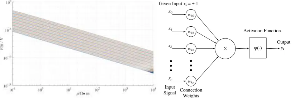
The induced electromotive force 𝑉(𝑡) = 𝑓(𝑡,ρ) is a non-linear complex function of resistivity ρ and sample time t. The apparent resistivity value is obtained from the measured EMF data, in fact that it is to find a reasonable resistivity value at a certain sample time. The resistivity value is calculated by Eq. (1) to be equal to the actual induced electromotive force or to Similar within the error. According to Eq. (1), Chen [12] calculated the induced electromotive force of time 𝑡 at 0.001, 0.01,

electromotive force value corresponds to a resistivity value at a certain sampling time window (or sampling time).

The idea of this paper is to establish a one-to-one correspondence between the induced electromotive force (EMF) sampled at a certain time and the resistivity value using ANN. It is to train the neural network structure with the EMF as the input and the resistivity value as the output using the fitting characteristics of the neural network. The apparent resistivity value of the measured EMF data is output directly at a certain sampling time using a trained neural network. The relationship between the induced electromotive force and the resistivity is established. And the neural network at each time window is established too. The induced electromotive force data collected by the receiver is substituted into the neural network of the certain time window, and the apparent resistivity value of measuring point at the certain time window is output directly. This method does not need to be recalculated or retrained, without iteration. It is simple and high precision.

Σ

wk0 Given Input x0 = ± 1

x0

x1

x2

xp

wk1

wk2

wkp Input

Signal Connection Weights

ψ(·) Activaion Function

yk Output

Figure 1. Variation of induced electromotive force with resistivity at each times window center.

Figure 2. The basic neuron model.

The Basic Principle and Formula Derivation of BP Neural Network

BP neural network is a multi-layer feedforward neural network composed of one input layer, one or more hidden layers and an output layer which all with fully interconnected neurons. The training process generally has two steps. Firstly, the forward process is to provide the training input value to the output layer. The second process (backpropagation process) is to minimizes the mean square error of network between actual and target outputs using the iterative gradient descent method (or the steepest descent method) according to the BP learning rule. For three-layered feedforward ANN, as Figure 2 shown, i over input neurons, j over hidden, o over outputs, the mean square error overall output layer neurons is written:

2 2

1 1

( ) [ ( ( ))]

2 o o o 2 o o j jo i ij i

E









(2)

do = target output of neuron o, oo = actual output of neuron o, wij = connection weights from the

input neuron i to the hidden neuron j, wjo = connection weights from the hidden neuron j to the output

neuron o.

We set up weight update of two arbitrary connected neurons m and n of neural network is the negative gradient of the energy function

mn

mn

E w

w  

  



(3) where, η is the learning rate, η∈ (0, 1); ∂E/∂wmn is the gradient of the energy function, which is a

vector containing the partial differential of weights. The optimal value of ∂ETotal/∂wmn is calculated

Levenberg-Marquardt Method. Gradient descent training to correct the weights, in order to reduce the oscillation of the weight change, the introduction of momentum α, as a change in the weight of the front coefficient, through the following iterative expression to achieve:

( 1) ( ) ( ) ( ) ( 1)

mn mn n m mn

w t w t  t t   w t ₍₄₎

where, α is the momentum term, α∈ (0,1). The weights are updated by the gradient descent method, loaded each sample and the weights updated once.

Design and Implementation of Calculation Apparent Resistivity with Neural Network

The output of receiver system is arithmetic intensive sampling at equal intervals. We set the time window of different widths, and divide the intensive sampling data into several delay channel windows. The sampling data within the same time window is overlaid and averaged. This can suppress the amplitude of random noise. The program is set so that the first window time is always equal to or larger than sample width. The number of windows and number of points per window are set by the receiver sample rate depending on the transmit frequency. The center of the time windows is determined by window time width (sampling delay) and turn-off time of transmitter system.

The input-output structure of the neural network is established for the correspondence between the induced electromotive force and the resistivity at the center of each time window. The apparent resistivity value is obtained by the induced electromotive force data of each measuring point at the center of the time window substituting into the built network at the center point of the time window. By analogy, the apparent resistivity values of all measuring points at all time-window centers are output by the neural network.

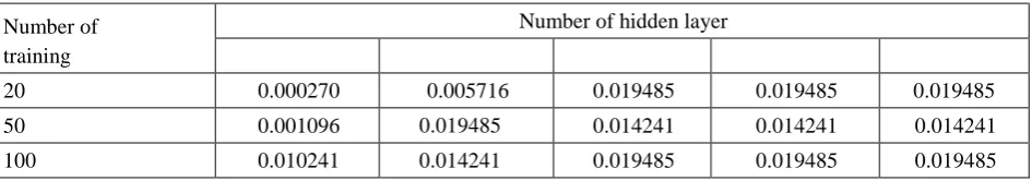
Table 1. The convergence of different hidden nodes in training. Number of

training

Number of hidden layer

20 0.000270 0.005716 0.019485 0.019485 0.019485

50 0.001096 0.019485 0.014241 0.014241 0.014241

100 0.010241 0.014241 0.019485 0.019485 0.019485

Firstly, the structure of the neural network, learning rules and training samples are determined. In this paper, three-layer feedforward neural network is selected. transient electromagnetic induction electromotive force is calculated according to Eq. (1), and a single-input-single output network structure is designed at a sampling time. There have been no generally valid solutions to the problem of determining hidden neurons. In this paper, we try to determine the number of neurons in the hidden layer by comparing the convergence errors of network structures with different numbers of neurons, as shown in Table 1. Finally, the three-layer feedforward neural network with single-input and single-output is established. The number of neurons in hidden layer is 12, and the learning rule is backpropagation.

structure randomly. The gradient descent algorithm is used to train the back propagation, and finally the neural network structure at sampling time t is obtained.

The ANN at each sampling time can be used as a general tool for solving the apparent resistivity of the transient electromagnetic field. The measured EMF data is input to the built ANN, and the apparent resistivity value corresponding to the induced EMF at the sampling time is mapped directly. The built ANN can be used to simulate all center loop transient EMF data, and quickly obtain the apparent resistivity value at a sampling time point. It is simple and quick, and save the iterative time consumed by the numerical solution.

Simulation Model of Transient Electromagnetic Grounding Network Detection

The simulation model of grounding grid break point is established. A large cube with a length of 100 m was used to simulate the uniform half-space, which is as soil with resistivity ρ = 50 Ω m. The ground grid was 0.8 m below surface of the soil model. Grounding grid model specifications are: meshes number 5 × 5, meshes size 6 m × 6 m, position of breakpoint is shown in Figure 4. Transmitter coil and receiver coil have a common center and were located directly above measuring point. Transmitter coil radius was 1.25 m, which was loaded a ramp pulse current which the peak current was 1 A and turnoff time was 100 μs. Receiver coil radius was 0.25 m.

：断点位置

3 9 15

-3 -9

-15 -15

-9 -3 3 9 15

X Y

(-9,13) (-7,13)

(4,-13) (6,-13) ：测点 1M

1M

：断点位置

3 9 15

-3 -9

-15 -15

-9 -3 3 9 15

X Y

(a) (b)

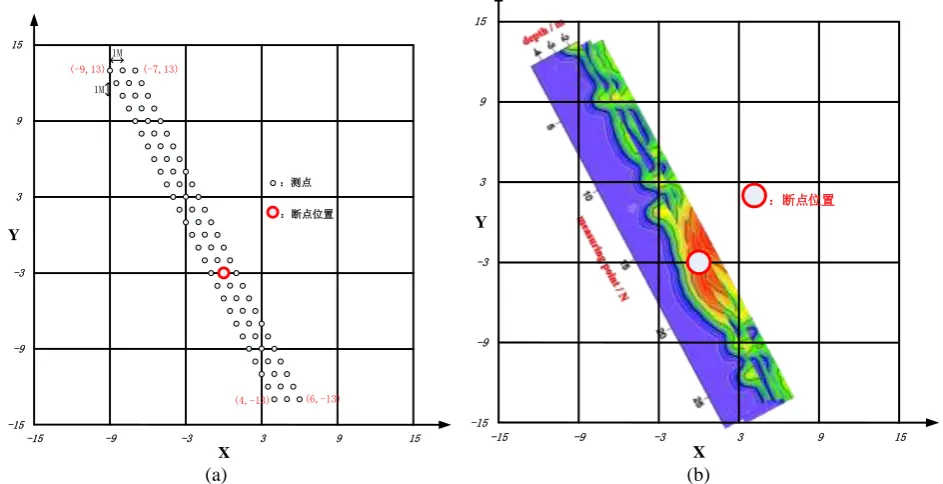
Figure 3. (a)The grounding grids structure model and position of breakpoint (coordinates (0, -3)) and measuring points. (b)Three-dimensional apparent resistivity contours slice display of grounding grids structure model.

As shown in Figure 3.(a), we selected a detection range that contained the breakpoint position, set line direction and measuring point spacing. 3 measuring lines crossed flat steel diagonally was set, the distance between the measuring points in X-axis direction was 1 m, and the measuring point spacing in Y-axis direction was 1 m. The distance between the measuring points which were right above the flat steel in the X-axis direction was 1 m, and in the y-axis direction was 2 m. The four vertex coordinates of the measuring range were (-9, 13), (-7, 13), (4, -13) and (6, -13), and the breakpoint position was at the (0, -3) coordinate.

distinguished using transient electromagnetism apparent resistivity scanned image. A high resistance patch is shown at the two grid grids where the breakpoint located, which makes it more intuitive to display breakpoint location.

The simulation model, which included eight lines, 27 measuring points per line, a total of 216 measuring points. This work needs to build 26 neural networks to fit the EMF data of all measuring points in each window. The built Neural network was seen as a mapping box, in which directly calculated the apparent resistivity of 216 measurement points at each sampling time. The time it takes for calculating and saving the result at a sample time window is 0.83 seconds (Inter (R) Core i7-3770K CPU3.50G 3.90GHz, RAM 16.0GB), which is much less than the numerical iteration of computation time. The proposed method is also suitable for systems of sending current frequencies at 4, 8, 16 and 32 Hz.

Conclusion

In this paper, a neural network is built based on the input of the induced electromotive force 𝑉(𝑡)and the output of the resistivity ρ for fitting the TEM apparent resistivity value at a sampling time according to the expression of the induced electromotive force (EMF) response and the characteristic that the induced electromotive force drops monotonously with the increase of the resistivity in the range of 0.08ms < 𝑡 < 1𝑠. The proposed method avoids the calculation of specific complex electromagnetic field or numerical inverse problem, thereby realizing the rapid resistivity calculation of TEM. The model is validated by the grounding grid, which is effective in identifying breakpoint and saving the computing time.

References

[1]S. H. Ward, G. W. Hohmann, Electromagnetic Theory for Geophysical Applications. Electromagnetic Methods in Applied Geophysics: Volume 1, Theory. Society of Exploration Geophysicists, 1988: 130-311.

[2]B. R. Spies, A. P. Raiche, Calculation of apparent conductivity for the transient electromagnetic (coincident loop) method using an HP-67 calculator. Geophysics, 1980, 45(7): 1197-1204.

[3]A. P. Raiche, B. R. Spies, Coincident loop transient electromagnetic master curves for interpretation of two-layer earths. Geophysics, 1981, 46(1): 53-64.

[4]N. B. Christensen, 1D imaging of central loop transient electromagnetic soundings. Journal of Environmental & Engineering Geophysics, 1995, 2(1): 53-66.

[5]Z. Fu, T. Sun, Q. Chen, et al, Transient electromagnetic apparent resistivity imaging for break point diagnosis of grounding grids. Transactions of China Electrotechnical Socity, 2008, 23(11): 15-21. (in Chinese)

[6]Mirko van der Baan, Christian Jutten. Neural networks in geophysical applications. Geophysics, 2000, 65(4): 1032-1047.

[7]Z. Fu, C. Yu, X. Hou, et al., Transient electromagnetic apparent resistivity imaging for break point diagnosis of grounding grids. Transactions of China Electrotechnical Socity, 2014, 29(9): 253-259. (in Chinese)

[8] M. N. Nabighian, Quasi-static transient response of a conducting half-space-An approximate repre- sentation. Geophysics, 1979, 44(10): 1700-1705.

[9]Q. Chen, Searching Algorithm for Full Time Apparent Resistivity from TEM Electromotive Force Data. Journal of Oil and Gas Technology, 2009, 31(2):45-49. (in Chinese)

[11]S. Yang. All-Time Resistivity Calculation in Consideration of Time-Off Using the Central Tem Loops Method. Geophysical and Geochemical Exploration, 2008, 32(6):647-651. (in Chinese)

[12]J. Li, T. Li, X. Zhao, et al., Study on the TEM all-time apparent resistivity of arbitrary shape loop source over the layered medium. Progress in Geophysics, 2007, 22(6):1777-1780. (in Chinese)

[13]H. Wang. Time domain transient electromagnetism all time apparent resistivity translation algorithm. Chinese J .Geophys., 2008, 51(6):1936-1942.(in Chinese)