The Parallel Solution Method of Sparse Triangular System Based on Correlation Decomposition

2018 International Conference on Information, Electronic and Communication Engineering (IECE 2018) ISBN: 978-1-60595-585-8

The Parallel Solution Method of Sparse Triangular System

Based on Correlation Decomposition

Li-cui SONG, Song JIN

and Tian-cheng LV

Department of Electronics and Communication Engineering, North China Electric Power University

*Corresponding author

Keywords: Parallel computing, The partial value of the variable, Multi-nuclear multithreading.

Abstract. We propose a parallel solution algorithm based on correlation decomposition. By decomposing the right-hand-side of the linear system and analyzing the dependencies of the variable solution to form multiple independent variable calculation paths. First, the partial value of the variable is calculated in parallel, and then the final result of the variable is calculated by adding the partial value of the variable. Since the variables are calculated without waiting for all the precursor variable to complete the calculation, which greatly improves the parallelism and calculation speed, and communication between multiple parallel tasks only once, which reduces synchronization overhead.

Introduction

The solution of sparse linear triangulation is one of the most important problems in many scientific calculations and engineering techniques. With the improvement of the scale and complexity of scientific and engineering problems, higher requirements are put forward for the solving scale and speed of the sparse triangular system [1]. At present, how to solve the sparse linear triangulation system quickly and efficiently has become the focus of research.

The rapid development of parallel computing technology provides new ideas and powerful tools to solve computationally intensive problems [2]. Sparse data structures lead to two opposite ways to partition data to solve the sparse linear triangulation solution in parallel: fine-grain partitioning and coarse-grain partitioning [3]. Coarse-grained parallel algorithm [4]: the lower triangular matrix is divided into blocks by columns, and calculated in parallel between the blocks, within a single block, the variable is solved in order of dependency. This method significantly improves the computational speed, but how to achieve an optimal blocking strategy is still a problem; fine-grained parallel algorithm [5]: the rows are divided into different layers by the dependency between the lower triangular matrix rows, and the different layers are sequentially executed, which the rows in the same layer are computed in parallel. This method effectively implements parallel solution, but frequent data transfer between layers makes communication overhead large. Aiming at the problems of the above parallel algorithms, we propose a parallel solution method based on correlation decomposition to achieve efficient solution of sparse triangle systems.

In this paper, the parallel algorithm is implemented on multi-cores processor [6]. A sparse linear triangulation system is constructed based on the Florida sparse matrix set [7], and solve by the proposed algorithm. The experimental results show that compared with Nvidia’s cuSPARSE library

[9]

, the proposed algorithm can increase the calculation speed by about 19%. Compared with the serial algorithm, the proposed algorithm can increase the calculation speed by about 72%.

Background

11 1 1

22 2 2

32 33 3 3

42 44 4 4

51 53 55 5 5

62 63 66 6 6

71 72 73 74 77 7 7

85 88 8 8

L x b

L x b

L L x b

L L x b

L L L x b

L L L x b

L L L L L x b

L L x b

                                   _{ }                                          

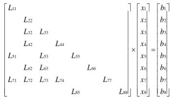
Figure 1. The sparse linear lower triangular system.

The direct method [8] solves the sparse linear lower triangular system with the Equation 1:

1

0

( ) / (0 8)

j

j j jk k jj

k

x b L x L j





 



It can be known from Equation 1 that there is an inherent dependence in solving sparse linear triangular systems. For example, if Lji is a non-zero value, then the calculation xj depends on the

precursor variablexi. According to the dependence relationship of variable solution, we can construct

a directed acyclic graph (DAG) represents the order of variable solution [9], as shown in Figure 2. In Figure 2: a circle represents a variable, and an arrow between two circles represents a direct dependency between two variable solutions.

1 2

3 4

5 6 7

8

Figure 2. DAG of the lower triangular matrix.

The Algorithm of Correlation Decomposition

Theory of Correlation Decomposition

Consider the sparse linear trigonometric system of Figure 1. If b1 is not 0 and the other

( 2,3 8)

i

b i  are 0, the process of calculating each variable by equation 1 is as follows:

1 1 11 2 3 4 5 5 51 1 53 3 55 51 1 55

7 7 71 1 72 2 73 3 77 71 1 77 8 8 85 5 88 85 5 88

/ 0 ( ) / /

( ) / / ( ) / /

x b L x x x x b L x L x L L x L

x b L x L x L x L L x L x b L x L L x L

           

               

From the above process of solving variables, we find that only when b1 is not 0, the partial value of the variables x x x x1、 5、 7、8 _{can be calculated. If} x1is calculated, the partial values of x x5、 7 _{can be} calculated simultaneously, and the partial value of x8 can be calculated by the partial value of x₅. Therefore, the above process of solving variables can be divided into two calculation processes.

Calculation process 1: x1 calculates x5 and thenx8is calculated byx5. Calculation process 2: x1 calculatesx7.

The two calculation processes can calculate the variable partial values in parallel. We refer to the divided calculation process as the variable calculation path. In summary, we propose a parallel solution method for linear trigonometric systems: set the right-hand-side b ii( 1, 28)to have only one

calculation paths is used to calculate the partial value of the variable in parallel, then all the values of the variables are added to calculate the final value of the variables.

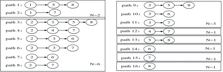
Taking the sparse linear trigonometric system of Figure 1 as an example, the parallel method proposed in this paper is applied to solve the problem. First, the process of solving the sparse linear triangulation system is divided into multiple variable calculation paths. Set the right-hand-side

( 1, 2 8) i

b i  of the sparse triangle system in turn, only one item is not 0. According to the dependence

relationship existing in the variable solution, the solution process is decomposed into 16 variable calculation paths, and the obtained paths are as shown in Figure 3.

6

7

8

1 5 8

2 path 1：

7

3 5 8

2

4 7

path 2：

path 3：

path 4：

path 5： 3 6

path 6： 2 3 7

2

path 7： 6

path 8： 2 7

2

path 9： 3 5 8

path 10： 3 6 1

path 11： 3 7 path 12： 4 7 path 13： 5 8

path 14：

path 15：

path 16：

N=2 N=6 N=3 N=1 N=1 N=1 N=1 N=1

Figure 3. The 16 variable calculation paths.

In Figure 3, we use N to represent the number of paths divided by the same variable; the variables

that pass through the path are called other related variables on this path, and are represented by the setU. For example, if b1is not 0, the variable x1 is used as the starting point, and two variable calculation paths are divided, N2, which are path 1 and path 2 in Figure 3 respectively; and the set of

other related variables on path 1 is U{7,8}, the set of other related variables on path 2 is U{5}.

After that, the partial values of the variables are calculated in parallel. The 16 variable calculation paths are distributed to 16 threads, and the variable partial values are calculated in parallel between threads; in a single thread, the variable partial value is calculated according to the dependency of the variable calculation path. Specific to a single thread, the partial values are calculated as equation 2 and equation 3:

/

i i ii

x b L (2)

( ) / ( )

j jk k jj

x   L x L jU ₍₃₎

In equation 2: the subscript iindicates the label of the starting point on a single path; in equation 3: the subscript j_{represents the variable number, and the subscript} krepresents the precursor variable label of the variable xj on a single path, and U is the other related variable on a single path set.

Finally, after the 16 variables are calculated in parallel, all the values of the variable

( 1, 2 8)

i

x i  are added, and the sum of the sums is divided by the number Nof the paths defined by

the variable x ii( 1, 28)as the starting point, and the final solution vector is calculated.

Implementation of Parallel Algorithm

Considering that the number of processors in the experimental platform is small, and the number of variable calculation paths is particularly large, this results in the serial processing of many variable calculation paths in a processor, which reduces the running speed. In order to reasonably match the number of divided paths and the number of processors, when implementing the parallel solution algorithm in this paper, the method of dividing the variables to calculate the path is as follows: sequentially setthe right-hand-side b ii( 1, 2,3.... )n of the sparse triangle system have _M terms are not

0, and start from Mstarting points and calculate the partial value of the variable. Then, Minitial values

other M1 starting values are calculated by equation 4; equation 3 is transformed into equation 5,

which calculates the partial values of other related variables within a single thread:

1

( ) / ( )

t

t t tk k tt t

k i

x b L x L t U





 



1

( ) / ( )

j

j jk k jj

k i

x L x L j U





 



In equation 4, the subscript t represents the other M1 starting variable numbers, and Ut is the set

of other M1 starting variables. In equation 5, the subscript j represents the variable number, and

U is a collection of other related variables within a single thread.

Implementation of the correlation decomposition algorithm. First, in the main function, the solution process of the sparse triangle system is divided into several calculating paths, and each calculation path is arranged by one thread’s calculation. For convenience of description, let the order of the triangular matrix L be n, the number of threads is set to p, andpcan be divided by n, mn p/ . The right-hand-side is divided into groups of m values, and the division result is shown in Fig. 4. Fig. 4 divides the right-hand-side into p blocks, each block is numbered0,1, 2,...p1, and each block is dispatched by the operating system into one thread for calculation, and all threads execute in parallel.

1 2 1 2 2 2 1 2 2 1

{ , , , , , , }

T

m m m m m m n m n n

b b b b b b b b b b b

B

m个值 m个值 …… m个值

Figure 4. Division of the right end item B.

Specific to a single thread, through the dependency of the variable solution, the last column is found from the starting column to form a variable calculation path, and the partial value of the variable is calculated simultaneously. The description of the calculation process within a single thread is shown in Figure 5.

Calculation within a single thread

INPUT: value, col_ind, row_ptr, Bi, i RETURN: x

1: x[i*m]=Bi[i*m]/value[i*m] /* calculates the first starting value */ 2: For t=i*m+1 TO t=(i+1)*m Do

3: For p=0 TO p=number Do /* number represents the number of predecessors of the variable xt in this thread*/ 4: SUM=value[ref_ptr[t]+p]*x[col_ind[ref_ptr[t]+p]]+SUM /* summation in Equation 6 */

5: EndFor

6: x[t]=(Bi[t]-SUM)/value[t] /* calculates the value of the other m-1 starting variables xt */ 7: EndFor

8: For j=(i+1)*m+1 TO j=n Do

9: For p1=0 TO p1=count Do /* count represents the number of previous variables of this thread variable xj_*/ 10: if x[col_ind [ref_ptr [j]+p1]]!=0 then

11: sum=sum-value[ref_ptr[j]+p1] /* x[col_ind[ref_ptr[j]+p1]] /* summation in Equation 7 */ 12: EndIf

13: EndFor

14: x[j]=sum/value[j] /* calculates the value of other related variables xj in this thread.*/ 15: EndFor

Figure 5. Description of the calculation process within the thread.

Then, after the p threads are calculated, all the calculation results are returned to the main function, and all the values of the variables are added to calculate the final solution vector.

Case Analysis

operating system, the Callable interface is applied to solve the sparse linear triangle system. And we evaluate our algorithm against the state-of-the-art cuSPARSE algorithm.

In this paper, a Florida matrix with different sparsity is used to form a sparse linear lower triangular system. Table 1 is a Florida matrix with a relatively small sparsity, and Table 2 is a Florida matrix with a very small sparsity.

Table 1. Florida matrix with less sparsity.

matrix name rows/columns sparsity(%)

pwtk 217918 0.02

SiO2 155331 0.047

shallow_water1 81920 0.69

finan512 74752 0.24

cant 62451 0.86

gridgena 48962 1.12

wathen100 30401 1.66

gyro_m 17361 8.39

Table 2. Florida matrix with very small sparsity.

matrix name rows/columns sparsity(%)

thermomech_dM 204316 0.0039

xenon2 157464 0.016

shallow_water1 81920 0.0061

finan512 74752 0.012

cant 62451 0.11

gridgena 48962 0.023

wathen100 30401 0.054

gyro_m 17361 0.34

Comparison of Algorithms

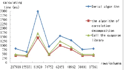
In this paper, we use the matrix with small sparsity in Table 1 and the matrix with very small sparsity in Table 2 to form a linear trigonometric system and solve it. In order to reflect the advantages of the proposed algorithm, run a 4-core processor and set 8 threads, and then compare the algorithm of correlation decomposition with the serial algorithm and the cuSPARSE algorithm. After many experiments, the results in Fig. 6 were obtained.

From the graph (a) in Figure 6, it can be clearly seen that compared with the serial algorithm and the cuSPARSE algorithm, the correlation decomposition algorithm has the smallest calculation time and the fastest calculation speed. Compared with the matrix adopted in graph (a), the matrix adopted in graph (b) has the same or similar order, but the sparsity decreases. The calculation time of the three methods are greatly reduced, however, compared with the serial algorithm and the cuSPARSE algorithm, the calculation time of the algorithm in this paper is still minimal, and the calculation speed is still the fastest.

(b) Calculating time for very sparse triangle systems

Figure 6. Calculating time comparison of three different algorithms.

It can be seen that whether the matrix of sparse degree is adopted in graph (a) or matrix of very small sparse degree is adopted in graph (b), the calculation speed of the correlation decomposition algorithm is obviously better than that of serial algorithm and the cuSPARSE algorithm.

Conclusion

In this paper, a sparse linear trigonometric system is constructed based on the Florida sparse matrix set, and the correlation decomposition algorithm is applied to solve those systems. Through comparison with the serial algorithm and the cuSPARSE algorithm, the efficiency of the parallel algorithm in this paper is verified.

Acknowledgements

The work was supported in part by Natural Science Foundation of Hebei province of China under Grant No. F2017502043.

References

[1]MB van Gijzen M B, Sleijpen G L G, Zemke J P M. Flexible and multi-shift induced dimension reduction algorithms for solving large sparse linear systems [J]. Numerical Linear Algebra with Applications, 2015, 22(1): 1-25.

[2]Ji C, Li Y, Qiu W, et al. Big data processing in cloud computing environments[C]//Pervasive Systems, Algorithms and Networks (ISPAN), 2012 12th International Symposium on. IEEE, 2012: 17-23.

[3]Picciau A, Inggs G E, Wickerson J, et al. Balancing locality and concurrency: solving sparse triangular systems on GPUs[C]//2016 IEEE 23rd International Conference on High-Performance Computing (HiPC). IEEE, 2016: 183-192.

[4]Mayer J. Parallel algorithms for solving linear systems with sparse triangular matrices [J]. Computing, 2009, 86(4): 291.

[5]Li A, van den Braak G J, Corporaal H, et al. Fine-grained synchronizations and dataflow programming on GPUs[C]//Proceedings of the 29th ACM on International Conference on Supercomputing. ACM, 2015: 109-118.

[6]Wang X, Xue W, Liu W, et al. swSpTRSV: a fast sparse triangular solve with sparse level tile layout on sunway architectures[C]//Proceedings of the 23rd ACM SIGPLAN Symposium on Principles and Practice of Parallel Programming. ACM, 2018: 338-353.

[8]Gould N I M, Scott J A, Hu Y. A numerical evaluation of sparse direct solvers for the solution of large sparse symmetric linear systems of equations [J]. ACM Transactions on Mathematical Software (TOMS), 2007, 33(2): 10.