SEQUENTIAL TESTING PROCEDURE AND THEIR ROBUSTNESS STUDY FOR ERLANG DISTRIBUTION

(1)

© Associated Asia Research Foundation (AARF)

A Monthly Double-Blind Peer Reviewed Refereed Open Access International e-Journal - Included in the International Serial Directories. Page | 222

SEQUENTIAL TESTING PROCEDURE AND THEIR ROBUSTNESS

STUDY FOR ERLANG DISTRIBUTION

Surinder Kumar, Vaidehi Singh and Prem Lata Gautam

Department of Statistics, School for Physical and Decision Sciences Babasaheb Bhimrao Ambedkar University, Lucknow, India-226025

ABSTRACT

The sequential testing procedures are developed for testing the hypotheses regarding the

shape and rate parameters of the Erlang distribution. Theoretical expression for the operating

characteristics (OC) and average sample number (ASN) functions are derived for these

parameters. The robustness of the SPRT'S in respect of OC and ASN functions are studied, when

the distribution under study has undergone a change. The acceptance and rejection regions for

0

H against H₁ are derived in case of rate parameter. The expressions of OC and ASN functions

for the robustness of the SPRT in case of rate parameter, when the coefficient of variation is

known are also derived and studied. Finally, the results are presented through Tables and

Graphs, so that one can see the numerical evaluated departures in OC and ASN functions.

Keywords: Erlang distribution, Sequential probability ratio test, Operating characteristics, Average sample number, Robustness, Coefficient of variation, Acceptance and rejection region.

International Research Journal of Natural and Applied Sciences

ISSN: (2349-4077) Impact Factor- 5.46, Volume 5, Issue 3, March 2018 Website- www.aarf.asia, Email : [email protected] , [email protected]

(2)

1. Introduction

The concept of sequential testing of statistical hypotheses for testing between two simple hypotheses is first developed by Wald (1947). This concept is heavily dominated by the sequential probability ratio test (SPRT). In order to study the performance of the SPRT’S, Wald (1947) derived the theoretical expressions for the operating characteristics (OC) and average sample number (ASN) functions. Sequential probability ratio test has been applied by several researchers, to tackle with different testing problems, for references one may referred to Oakland (1950), Epstein and Sobel (1955), Johnson (1966), Phatarford (1971), Bain and Engelhardt (1982), Chaturvedi et al. (2000), Sevil and Demirhan (2008).

The robustness of the SPRT in respect of OC and ASN functions has been studied by several authors, when the distribution under consideration has undergone a change, while dealing with various probabilistic models. For references, Harter and Moore (1976) gives sampling plans for reliability tests under the assumption of a constant failure rate and by using Monte Carlo techniques, the robustness of the exponential SPRT is studied, when the underlying distribution is a Weibull distribution. Montagne and Singpurwalla (1985) investigated the robustness of the sequential life-testing procedure with respect to the risks and the expected sample sizes for the exponential distribution when the life length is not exponential. Hubbard and Allen (1991) applied SPRT on the mean of the negative binomial distribution when the dispersion parameter is known and the robustness of the test to the misspecification of dispersion parameter is studied. Chaturvedi et al. (1998) considered a family of life-testing models and studied the robustness of the SPRT’S for various parameters involved in the model and also generalised the results of Montagne and Singpurwalla (1985).

Joshi and Shah (1990) developed SPRT for testing a simple hypothesis (against a simple alternative) for the mean of an inverse Gaussian distribution, assuming the coefficient of variation (CV) to be known. They obtained theoretical expressions for the OC and the ASN functions.

(3)

2. Set up a problem:

Let us consider a random variable (r.v.) X follows the Erlang distribution presented by the probability density function (pdf)





! ) 1 -( ,

;

1 k

e x k

x f

x k k 



    ; 0x, 0, kN (2.1)

where k is the shape parameter and λ is the rate parameter. The Erlang distribution is the sum of ‘k ’ independent exponential random variables each with the same parameter. For a given

sequence of observations X₁, X₂, X₃… from (2.1), the problem of testing the simple null hypo-

thesis H₀:₀ against the simple alternative hypothesis H₁:₁(₀) is considered.

In Section 3, 4, 5, 6 and 7, respectively, we develop the SPRT’S for the parameters involved in the model (2.1). The robustness of the SPRT’S in respect of OC and ASN functions, when the distribution under consideration has undergone a change is studied [see Remarks 3.1, 4.1, 5.1, 6.1]. Also, the robustness of the SPRT for a mis-specified coefficient of variation is studied in Section 7[see Remarks 7.1]. In Section 8, the acceptance and rejection regions for H0 vs H1 in case of λ are derived and plotted in Figure 8.1. Finally, in Section 9, the results and findings are presented through Tables and Graphs.

3. SPRT for testing the hypothesis regarding ‘λ’

The SPRT for testing H0:0 against H1: 1(1 0) is defined as follows









_ 

  

k x f

k x f Z

i i i

, ;

, ; ln

0 1  

(3.1)



₀ ₁



0 1

ln  



 _ _

     

 _i

i k x

Z (3.2)

We choose two numbers A and B such that 0B1A. At the nth stage of sampling accept H₀if



 

n i

i

z

1

lnB, rejectH₀ if



 

n i

i

z

1

lnA, otherwise continue sampling by taking the

(4)

A Monthly Double-Blind Peer Reviewed Refereed Open Access International e-Journal - Included in the International Serial Directories. Page | 225 



 1

A and

 

 

1

B (3.3)

The Operating Characteristic (OC) Function L()is given by

h h h B A A    1 )

L( (3.4)

where ‘h’ is the non-zero solution of

 

_eZi h 1

E (3.5)

or, 1 ) , ; ( ) , ; ) , ; ( h 0 0 1       



 f x k dx

k f(x k x f i i i    (3.6)

From (2.1) and (3.2), we obtain

k h kh h Zi e E    _ _        ) ( 1 0 1 1 0 ] [      (3.7)

Finally, from equation (3.5) we get

h h          0 1 1 0 1 ) (    

 (3.8)

This expression (3.8), is not useful for finding the values of OC and ASN functions, hence, in order to tackle this problem we take the logarithm of both sides and using the

expansion ; 1 1

3 2 ) 1 ln( 3 2       

x x x x x and retaining the term up to third degree in ‘h’,

we get





                        

 ₀ ₁

0

1 _ln₁

ln k h

kh                                        3 1 0 3 2 1 0 2 1 0 0 1 3 2 ln          

 h h

(5)

A Monthly Double-Blind Peer Reviewed Refereed Open Access International e-Journal - Included in the International Serial Directories. Page | 226 or 0 ln 2 3 ₀ 1 1 0 2 1 0 3 1 0 2                                           h h (3.9)

which is a quadratic equation in ‘h’. On solving (3.9), we get the real roots of ‘h’. Finally, on substituting the values of ‘h’ in equation (3.4) the numerical values of OC function are obtained. The ASN function is approximately given by





) ( ln ) ( 1 ln ) ( ) / ( Z E A L B L N

E       (3.10)

provided that E(Z)≠0, where

                        

 0 1

0 1 ln )

(Z k

E (3.11)

From equation (3.11), the ASN function under H0 and H1 is given by

                              1 0 0 1 0 ln ln ln ) 1 ( ) ( k A B N

E (3.12)

and                               1 0 0 1 1 ln ln ) 1 ( ln ) ( k A B N

E (3.13)

Remarks 3.1: Let us consider the problem of testing the simple null hypothesis H₀ :₀ 13

(6)

4. Robustness of the SPRT for ‘λ’when ‘k’ has undergone a change

Let us suppose that the parameter ‘k’ has undergone a change to k*and then probability distribution in (2.1) becomes f(x;,k*). In order to study the robustness of SPRT developed in Section 3 with respect to OC function, the values of ‘h’are obtained by solving the following

1 ) , ; ( ) , ; ( ) , ; ( * 0 , 0 1         



 f x k dx

k x f k x f i h i i    (4.1) 1 ) 1 ( 0 )] ( [ * 0

1 0 1 *

*          _   



e x dx

k k h x k kh      

Finally, we get

1 1 * 1 0 0 1                    

 kh k

h      (4.2)

taking logarithm on both sides of equation (4.2) and using the expression of ln(1-x), x 1. In

order to obtain the roots of the given equation and retain the terms upto third degree in ‘h’ we get the following quadratic equation

0 ln 2 3 ₀ 1 1 0 2 1 0 3 1 0 2                                           p hp p h

, (4.3)

where k k p * 

which is quadratic equation in ‘h’. On solving, we get the real roots of ‘h’. The Robustness of the SPRT with respect to ASN is studied by replacing the denominator of (3.10) by



Z



z f x k dx

E



  0 * ) , ; (  





( ₀ ₁) ( )

0

1 _E _x

In k Z

E  

   _       





_                   

 0 1 *

(7)

, ln

)

( 0 1

0 1                      p Z E (4.4)

Remarks 4.1: For testing the simple null hypothesis H0:0 13against the simple alternative

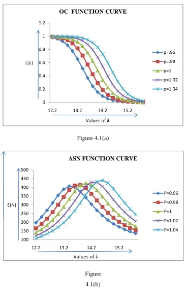
hypothesis H1:115for   0.05 for different values of 'k' the real roots of ‘h’ are obtained from equation (4.3). From Table 4.1(a) and Table 4.1(b), the values of OC and ASN curves are plotted in Figure 4.1 (a) and Figure 4.1 (b) for various values of 'p' . The OC curve

shifts to the left (right) and ASN curve shifts to the left downward (right upward) for p1(p >1). From both the curves, it is evident that the SPRT is highly sensitive for any change in ‘k’.

5. SPRT for testing the hypothesis regarding 'k'

Let the sequence of observation X₁, X₂, X₃… from (2.1). Our goal is to test the simple

null hypothesis H₀:kk₀ against the simple alternative hypothesis H₀:kk₁(k₁k₀).The

SPRT for testing H₀ is defined as follows:

Let (5.1) ) , ; ( ) , ; ( ln 0 1        k x f k x f Z i i i _ 

_i k k k k x_i

k k

Z ln ( ₁ ₀)ln ( ₁ ₀)ln

1

0    

       

  (5.2)

For OC curve we have

1 ) , ; ( ) , ; ( ) , ; ( 0 0 1       



 f x k dx

k x f k x f i h i i    (5.3)

From (2.1) and (5.2)



( )



1

0 1 1

0    

(8)

A Monthly Double-Blind Peer Reviewed Refereed Open Access International e-Journal - Included in the International Serial Directories. Page | 229 This expression (5.4) is not useful for finding the values of OC and ASN functions, hence we further calculate and taking the logarithm of both sides and using the approximation

(5.5) ln 2 1 2 ln

ln x x x  x

           we have 0 ) ( 2 1 ln 1 ln 2 1 ln 2 1 ) 1 2 ( 4 ) 1 4 (

12 0 0 1 1 1 0

2 0 1 3 0 1 2         _ _                _                   k k k k k k k k k k k k h k k k k h (5.6)

which is quadratic equation in ‘h’. On solving, we get the real roots of ‘h’. The numerical values of OC function is now obtain from equation (5.6). The Robustness of the SPRT with respect to ASN is studied by replacing the denominator of (3.10) by



Zi k



ln k0 ln k1 (k1 k0)ln (k1 k0)E(lnxi)

E        

and

 ( ) ln )

(Inx  k 

E i

Using the result of Gradshteyn and Ryzhik (1965, p.576 § 4.352(1)) that

(5.7) 2 1 ln ) ( x x

x  

 ) 8 . 5 ( ) ( 2 1 ln 1 ln 2 1 ln 2 1 )

( ₀ ₀ ₁ ₁ k₁ k₀

k k k k k k k Z

E _i  

     _ _                _ 

Remarks 5.1: Let us consider the problem of testing the simple null hypothesis H0 :k0 13

(9)

6. Robustness of the SPRT for ‘k’ when ‘λ’ has undergone a change

Let us suppose that the parameter ‘λ’ has undergone a change to λ*

and then probability distribution in (2.1) becomes f(x;*,k).In order to study the robustness of SPRT developed in Section 5 with respect to OC function, the values of ‘h’are obtained by solving the following



        0 * 0

1 ₍ _; _, ₎ ₁

) , ; ( ) , ; ( dx k x f k x f k x f i h i i    (6.1) 1 1 0 1 ) ( * ) ( 1

0 1 0 1 0 * 

        



      dx e x k k

k h _h _k _k k _h_k _k _k __x

 

Finally, we get



( )



1

1 0 1 ) ( 1

0 1 0    

          k k k h k k

k h k k

h

 (6.2)

where _* 

  

taking logarithm on both sides of equation (6.2) and using the approximation (5.5). In order to obtain the roots of the given equation and retain the terms upto third degree in ‘h’ we get the following quadratic equation

(6.3) 0 ) ( 2 1 ln 1 ln ) ( ln 2 1 ln 2 1 ) 1 2 ( 4 ) 1 4 ( 12 0 1 0 1 1 1 0 0 2 0 1 3 0 1 2         _ _                  _                         k k k k k k k k k k k k k k h k k k k h _

which is quadratic equation in ‘h’. On solving, we get the real roots of ‘h’. The numerical values of OC function is now obtain from equation (6.3). The Robustness of the SPRT with respect to ASN is studied by replacing the denominator of (3.10) by



Zi k



In k0 In k1 (k1 k0)In (k1 k0)E(lnxi)

E        

where * ln ) ( )

(ln x  k  

E _i

(10)

(6.4) ) ( 2 1 ln ln 1 ln 2 1 ln 2 1 )

( * ₀ ₀ ₁ ₁ k₁ k₀

k k k k k k Z

E _i 

      _ _ _                   

Remarks 6.1: For testing the simple null hypothesis H₀:k₀ 13against the simple alternative

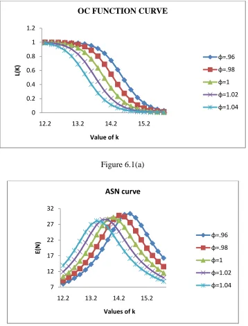
hypothesis H1:k115for   0.05 for different values of 'k' the real roots of ‘h’ are obtained from equation (6.3). From Table 6.1(a) and Table 6.1(b), the values of OC and ASN curves are plotted in Figure 6.1 (a) and Figure 6.1 (b) for various values of' ' . The OC curve shifts to the right (left) and ASN curve shifts to the right upward (left downward) for 1(1 ). From both the curves, it is evident that the SPRT is highly sensitive for any change in ‘k’.

7. Robustness of the SPRT for ‘λ’ with known coefficient of variation (CV)

For Erlang distribution mean and variance are

 

k  and(k 2), respectively then coefficient of

variation (CV) =(1 k). Let us suppose that coefficient of variation changes from a to a*, so that, the (pdf) of (2.1) shifts to f(xi;,a*).

Then OC and ASN function is

From (3.2) and (2.1)

(7.2) 1 ) ( 2 * 2 1 1 0 0 1                     a a h

h  

  



taking logarithm on both sides of equation (7.2) and using the expression of ln(1-x), x 1.In order to obtain the roots of the given equation and retain the terms upto third degree in ‘h’ we get the following quadratic equation

(11)

A Monthly Double-Blind Peer Reviewed Refereed Open Access International e-Journal - Included in the International Serial Directories. Page | 232 which is quadratic equation in ‘h’. On solving, we get the real roots of ‘h’. The numerical values of OC function is now obtain from equation (7.3). The Robustness of the SPRT with respect to ASN is studied by replacing the denominator of (3.10) by

   



 

       

   



 0 1

0 1 ln )

(Z Q

E

(7.4)

Remarks 7.1: For testing the simple null hypothesis H₀:₀ 13 against the simple alternative

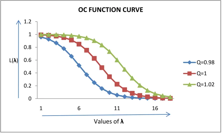
hypothesis H1:115for   0.05 for different values of '' the real roots of ‘h’ are obtained from equation (7.3). From Table 7.1(a) and Table 7.1(b), the values of OC and ASN curves are plotted in Figure 7.1 (a) and Figure 7.1 (b) for various values of ‘Q’. The OC curve shifts to the left (right) and ASN curve shifts to the left downward (right upward) for Q1(

1



Q ). From both the curves, it is evident that the SPRT is highly sensitive for any change in ‘λ’.

8. Implementation of Erlang distribution

We wish to test the simple hypothesis H0 :0against H1: 1(1 0)having

pre-assigned0 , 1. Let

) -(1 B and ) 1 (

  

 _

 

A and is defined as

) (

In ₀ ₁

0

1  



 _ _

     

 _i

i k x

Z

Let us defined,





 n

i i

X n

Y

1 )

( and N= first integer n ( ≥1) for which the inequality

dn c n

Y( ) 1 or Y(n)c2 dnholds with the constants

) (

ln ,

) (

ln ,

) (

ln

1 0

0 1

1 0 2 1 0

1 _ _

 

  

 

     

 



k

d A c

B

c (8.1)

Remarks 8.1: The figure (8.1) shows the acceptance and rejection regions for H₀under the case

(12)

A Monthly Double-Blind Peer Reviewed Refereed Open Access International e-Journal - Included in the International Serial Directories. Page | 233 ,

472 . 1 1

c c2 1.472 and d 0.1431, respectively. Thus, if Y(N)0.1434N1.472, we accept H₀ and if Y(N)0.1434N1.472, we accept H₁. At the intermediate stages, we continue sampling.

[image:12.612.68.541.138.309.2]

9. Tables and Figures

TABLE 3.1: OC and ASN Function

) 05 . 0 15,

: H , 13 :

(H0 0  1 1  

 L(λ) E(N)  L(λ) E(N)

12.2 0.9971 140.4986 14.2 0.3417 413.3708

12.4 0.9936 159.8104 14.4 0.2248 384.7040

12.6 0.9869 183.4731 14.6 0.1399 346.8554

12.8 0.9744 212.4760 14.8 0.0837 307.7820

13.0 0.9518 247.6194 15.0 0.0488 272.0115

13.2 0.9127 288.8578 15.2 0.0281 241.2071

13.4 0.8491 334.0960 15.4 0.0160 215.4333

13.6 0.7539 377.7574 15.6 0.0090 194.0947

13.8 0.6274 410.6952 15.8 0.0051 176.4329

14.0 0.4825 423.6839

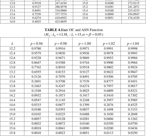
TABLE 4.1(a): OC and ASN Function

) 05 . 0 15,

: H , 13 :

(H0 0  1 1  

 p0.96 p0.98 p1.00 p1.02 p1.04

12.2 0.9780 0.9916 0.9971 0.9991 0.9998

12.4 0.9579 0.9830 0.9936 0.9978 0.9993

12.6 0.9228 0.9671 0.9869 0.9952 0.9984

12.8 0.8647 0.9388 0.9744 0.9900 0.9964

13.0 0.7762 0.8910 0.9518 0.9802 0.9924

13.2 0.6555 0.8153 0.9127 0.9622 0.9847

13.4 0.5126 0.7070 0.8491 0.9306 0.9705

13.6 0.3691 0.5708 0.7539 0.8777 0.9451

13.8 0.2463 0.4247 0.6274 0.7957 0.9017

14.0 0.1548 0.2916 0.4825 0.6809 0.8321

14.2 0.0932 0.1873 0.3417 0.5410 0.7302

14.4 0.0547 0.1145 0.2248 0.3957 0.5985

14.6 0.0315 0.0677 0.1399 0.2676 0.4525

14.8 0.0180 0.0393 0.0837 0.1698 0.3153

15.0 0.0102 0.0225 0.0488 0.1030 0.2048

15.2 0.0057 0.0128 0.0281 0.0606 0.1262

15.4 0.0032 0.0072 0.0160 0.0350 0.0750

15.6 0.0018 0.0041 0.0090 0.0200 0.0436

[image:12.612.66.541.230.679.2]

(13)

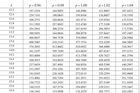
A Monthly Double-Blind Peer Reviewed Refereed Open Access International e-Journal - Included in the International Serial Directories. Page | 234 TABLE 4.1(b):_{OC and ASN Function}

) 05 . 0 15,

: H , 13 :

(H0 0  1 1  

 p0.96 p0.98 p1.00 p1.02 p1.04

12.2 _197.1554 _164.9055 _140.4986 _121.8907 _107.4472

12.4 _229.7191 _190.0843 _159.8104 _136.8897 _119.3350

12.6 _268.2753 _220.8636 _183.4731 _155.0764 _133.5339

12.8 _311.3303 _257.8043 _212.4760 _177.3108 _150.6794

13.0 _354.2941 _300.2334 _247.6194 _204.5853 _171.5784

13.2 _388.9491 _344.8844 _288.8578 _237.8447 _197.1987

13.4 _406.0037 _384.7538 _334.0960 _277.4993 _228.5586

13.6 _400.7087 _410.2143 _377.7574 _322.4249 _266.3805

13.8 _376.3043 _413.8602 _410.6952 _368.4888 _310.3017

14.0 _341.2197 _395.7450 _423.6839 _407.6247 _357.5151

14.2 _303.6089 _363.0557 _413.3708 _429.7627 _401.3790

14.4 _268.5015 _324.8010 _384.7040 _428.4458 _431.9220

14.6 _237.9659 _287.4981 _346.8554 _405.5380 _440.2997

14.8 _212.2997 _254.3281 _307.7820 _369.4382 _424.8342

15.0 _191.0183 _226.1628 _272.0115 _329.2599 _392.0868

15.2 _173.4081 _202.7294 _241.2071 _291.0522 _351.7520

15.4 _158.7723 _183.3453 _215.4333 _257.5169 _311.4459

15.6 _146.5152 _167.2734 _194.0947 _229.2211 _275.1647

15.8 _136.1561 _153.8588 _176.4329 _205.7377 _244.1852

Table 5.1: OC and ASN Function ) 05 . 0 15,

: H , 13 :

(H0 k0  1 k1   

k L(k) E(k) k L(k) E(k)

12.0 0.9994 9.2375 14.0 0.4909 29.2605

12.2 0.9983 10.3343 _14.2 _0.3502 _28.2711

12.4 0.9957 11.6721 _14.4 _0.2335 _26.0919

12.6 0.9903 13.3148 _14.6 _0.1481 _23.3677

12.8 0.9793 15.3305 _14.8 _0.0909 _20.6218

13.0 0.9583 17.7702 _15.0 _0.0548 _18.1363

13.2 0.9208 20.6176 _15.2 _0.0327 _16.0063

13.4 0.8581 23.7009 _15.4 _0.0194 _14.2266

13.6 0.7631 26.5972 _15.6 _0.0115 _12.7524

[image:13.612.67.549.88.410.2]

(14)

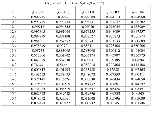
Table 6.1(a): OC and ASN Function

) 05 . 0 15,

: H , 13 :

(H₀ k₀  ₁ k₁   

k  .096 0.98  1.00  1.02  1.04

12.2 0.999945 0.9996 0.998309 0.994513 0.984968

12.4 0.999745 0.998784 0.995741 0.987647 0.968782

12.6 0.99918 0.996855 0.99026 0.974054 0.938909

12.8 0.997805 0.992664 0.979255 0.948609 0.887357

13.0 0.994749 0.984108 0.958327 0.903873 0.805774

13.2 0.988391 0.967552 0.920781 0.831233 0.690689

13.4 0.975849 0.93721 0.858111 0.725164 0.550266

13.6 0.95235 0.885095 0.763090 0.590112 0.404904

13.8 0.910806 0.802902 0.636174 0.443707 0.276973

14.0 0.842629 0.687288 0.490931 0.309185 0.17894

14.2 0.741441 0.54661 0.350214 0.202464 0.111184

14.4 0.609813 0.401403 0.233488 0.12688 0.067465

14.6 0.463623 0.273985 0.148072 0.077353 0.040411

14.8 0.326145 0.176626 0.090898 0.046434 0.024058

15.0 0.215002 0.109515 0.054752 0.027661 0.014292

15.2 0.135245 0.066319 0.032657 0.016428 0.008491

15.4 0.082572 0.039648 0.019396 0.009753 0.00505

15.6 0.049562 0.023561 0.011508 0.005796 0.003009

15.8 0.029493 0.013972 0.006832 0.00345 0.001796

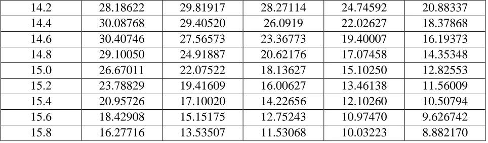
Table 6.1(b): OC and ASN Function

) 05 . 0 15,

: H , 13 :

(H₀ k₀  ₁ k₁   

k  0.96 0.98  1.00  1.02  1.04

12.2 8.052826 9.070382 10.33428 11.9178 13.89641

12.4 8.870748 10.11046 11.67214 13.64174 16.08068

12.6 9.848712 11.37437 13.31481 15.75179 18.67666

12.8 11.03152 12.92305 15.33047 18.28361 21.59022

13.0 12.47603 14.82574 17.77018 21.18239 24.51754

13.2 14.25006 17.14521 20.61763 24.20702 26.90107

13.4 16.42349 19.89954 23.70091 26.85593 28.09234

13.6 19.04171 22.98667 26.59718 28.46045 27.73625

13.8 22.06654 26.08093 28.65254 28.53432 26.03132

[image:14.612.64.554.48.418.2] [image:14.612.68.548.442.685.2]

(15)

14.2 28.18622 29.81917 28.27114 24.74592 20.88337

14.4 30.08768 29.40520 26.0919 22.02627 18.37868

14.6 30.40746 27.56573 23.36773 19.40007 16.19373

14.8 29.10050 24.91887 20.62176 17.07458 14.35348

15.0 26.67011 22.07522 18.13627 15.10250 12.82553

15.2 23.78829 19.41609 16.00627 13.46138 11.56009

15.4 20.95726 17.10020 14.22656 12.10260 10.50794

15.6 18.42908 15.15175 12.75243 10.97470 9.626742

15.8 16.27716 13.53507 11.53068 10.03223 8.882170

TABLE 7.1(a): OC and ASN Function

) 05 . 0 15,

: H , 13 :

(H₀ ₀  ₁ ₁   

 Q0.98 Q1.00 Q1.02

12.4 0.9586 0.9936 0.9994

12.6 0.9240 0.9869 0.9984

12.8 0.8667 0.9744 0.9964

13.0 0.7792 0.9518 0.9925

13.2 0.6592 0.9127 0.9850

13.4 0.5167 0.8491 0.9710

13.6 0.3729 0.7539 0.9460

13.8 0.2493 0.6274 0.9032

14.0 0.1569 0.4825 0.8345

14.2 0.0946 0.3417 0.7335

14.4 0.0555 0.2248 0.6025

14.6 0.0320 0.1399 0.4566

14.8 0.0182 0.0837 0.3188

15.0 0.0103 0.0488 0.2074

15.2 0.0058 0.0281 0.1279

15.4 0.0033 0.0160 0.0761

15.6 0.0018 0.0090 0.0443

[image:15.612.66.548.36.178.2]

(16)

TABLE 7.1(b): OC and ASN Function

) 05 . 0 15,

: H , 13 :

(H0 0  1 1  

 Q0.98 Q1.00 Q1.02

12.4 228.8271 159.8104 119.0274

12.6 267.2400 183.4731 133.1591

12.8 310.2311 212.476 150.2185

13.0 353.3110 247.6194 171.0078

13.2 388.3445 288.8578 196.4914

13.4 405.9958 334.096 227.6898

13.6 401.3142 377.7574 265.3421

13.8 377.3283 410.6952 309.1318

14.0 342.4041 423.6839 356.3408

14.2 304.7624 413.3708 400.4402

14.4 269.5302 384.7040 431.5077

14.6 238.8440 346.8554 440.5719

14.8 213.0351 307.7820 425.7066

15.0 191.6314 272.0115 393.2965

15.2 173.9209 241.2071 353.0365

15.4 159.2045 215.4333 312.6427

15.6 146.8827 194.0947 276.2077

[image:16.612.68.545.67.504.2]

(17)

A Monthly Double-Blind Peer Reviewed Refereed Open Access International e-Journal - Included in the International Serial Directories. Page | 238 Figure 3.1(a)

Figure 3.1(b) 0

0.2 0.4 0.6 0.8 1 1.2

12.2 13.2 14.2 15.2

L (λ)

Values of λ

OC FUNCTION CURVE

140 190 240 290 340 390 440

12.2 13.2 14.2 15.2

E(N)

Values of λ

[image:17.612.130.484.7.597.2] [image:17.612.131.482.45.257.2]

(18)

[image:18.612.123.491.28.629.2] [image:18.612.128.487.45.318.2]

Figure 4.1(b)

0 0.2 0.4 0.6 0.8 1 1.2

12.2 13.2 14.2 15.2

L(λ)

Values of λ

p=.96

p=.98

p=1

p=1.02

p=1.04

100 150 200 250 300 350 400 450 500

12.2 13.2 14.2 15.2

E(N)

Values of λ

ASN FUNCTION CURVE

P=0.96

P=0.98

P=1

P=1.02

(19)

Figure 5.1(b) 0

0.2 0.4 0.6 0.8 1 1.2

12 13 14 15

L(K)

Values of k OC FUNCTION CURVE

8 13 18 23 28 33

12 13 14 15

E(N)

[image:19.612.127.484.41.540.2] [image:19.612.127.487.45.256.2]

(20)

Figure 6.1(b) 0

0.2 0.4 0.6 0.8 1 1.2

12.2 13.2 14.2 15.2

L(K

)

Value of k

φ=.96

φ=.98

φ=1

φ=1.02

φ=1.04

7 12 17 22 27 32

12.2 13.2 14.2 15.2

E(N

)

Values of k

ASN curve

φ=.96

φ=.98

φ=1

φ=1.02

[image:20.612.129.487.35.505.2]

(21)

Figure 7.1(b) 0

0.2 0.4 0.6 0.8 1 1.2

1 6 11 16

L(λ)

Values of λ OC FUNCTION CURVE

Q=0.98

Q=1

Q=1.02

100 150 200 250 300 350 400 450 500

12.4 13.4 14.4 15.4

E(N)

Values of k

ASN FUNCTION CURVE

Q=0.98

Q=1

[image:21.612.125.488.68.291.2] [image:21.612.126.487.77.575.2]

(22)

A Monthly Double-Blind Peer Reviewed Refereed Open Access International e-Journal - Included in the International Serial Directories. Page | 243 Figure 8.1

REFERENCES

1 Bacanli, S. and Demirhan, Y. P. (2008): A group sequential test for the Inverse Gaussian Mean Statistical Papers, 49, 337-386.

2 Bain, L. J. and Engelhardt, M. (1982): Sequential Probability Ratio Tests for the shape parameter of NHPP, IEEE Transaction on Reliability, R-31, 79-83.

3 Chaturvedi, A., Kumar, A. and Surinder, K. (1998): Robustness of the sequential procedures for a family of life-testing models. Metron, 56, 117-137.

4 Chaturvedi, A., Kumar, A. and Surinder, K. (2000): Sequential testing procedures for a class of distributions representing various life testing models. Statistical papers, 41, 65-84.

5 Chaturvedi, A., Tiwari, N., and Tomer, S. (2002): Robustness of the sequential testing procedure for the generalized life distribution. Brazilian Journal of Probability and Statistics , 16, 7-24.

-2 -1 0 1 2 3 4 5 6

0 5 10 15

Y(N)

Accept H₀

ACCEPTANCE AND REJECTION REGION

L1

L2

Continue sampling Reject H₀

(23)

6 Epstein, B. and Sobel, M. (1955): Sequential life tests in exponential case. Ann. Math. Statist., 26, 82-93.

7 Gradshteyn, I.S and Ryzhik, I.M (1980): Tables of integrals, Series and Products Academic Press, London.

8 Harter, L. and Moore, A. H. (1976): An evaluation of the exponential and Weibull test plans. IEEE Transaction on Reliability, 25, 100-104.

9 Hubbard, D. J. and Allen, O. B. (1991): Robustness of the SPRT for a negative binomial to misspecification of the dispersion parameter. Biometrics, 47, 419-427.

10 Johnson, N. L. (1966): Cumulative sum control chart and the Weibull Distribution. Technometrics, 8, 481-491.

11 Joshi, S. and Shah, M. (1990): Sequential Analysis applied to testing the mean of an inverse Gaussian distribution with known coefficient of variation. Commun. Statist.-Theor. Meth., 19(4), 1457-1466.

12 Montagne, E. R. and Singpurwalla, N. D. (1985): Robustness of sequential exponential life-testingprocedures. Jour. American Statist. Assoc., 391, 715-719.

13 Oakland, G. B. (1950): An application of sequential analysis to whitefish sampling. Biometrics, 6, 59-67.

14 Phatarfod, R. M. (1971): A sequential test for Gamma distribution. Jour. American Statist. Assoc., 66, 876-878.