The bounds estimate of sub band operators for multi band wavelets

(1)

R E S E A R C H

Open Access

The bounds estimate of sub-band

operators for multi-band wavelets

Qingyun Zou

1*

_{, Guoqiu Wang}

2

_{and Qian Cao}

1,2

*_{Correspondence:}

qyzou2000@sina.com

1_{Hunan Province Cooperative}

Innovation Center for The Construction Development of Dongting Lake Ecological Economic Zone, Hunan University of Arts and Science, Changde, P.R. China Full list of author information is available at the end of the article

Abstract

A concept of the sub-band operator of multi-band wavelets is introduced, the theory of d-circular matrices is developed and the upper bound and the lower bound of the norm of the sub-band operator are obtained. Examples are provided to illustrate the results proposed in this paper.

MSC: 42C40; 42A16

Keywords: Multi-band wavelets; Circular matrix; Biorthogonality; Sub-band operators; Bounds estimate

1 Introduction

During the last three decades, the theory of frames, which generalize the notion of bases by allowing redundancy yet still providing a reconstruction formula, has been growing rapidly, since several new applications such as nonlinear sparse approximation (e.g., image compression), coarse quantization, data transmission with erasures, and wireless commu-nication, have been developed [1–7]. As a special class of frames, the multi-band wavelets have attracted considerable attention due to their richer parameter space, to give better energy compaction than 2-band wavelets [8–16].

LetHbe a separable Hilbert space, andEan indexing set. A sequence{fl}l∈Eis called a frame inHif there exist constants 0 <A≤B< +∞such that

Af2≤ l∈E

f,fl 2

≤Bf2, ∀f∈H, (1.1)

whereAandBare called lower and upper frame bounds, respectively. IfA=B, the frame is called tight frame.

WhenH=L2_{(R), a wavelet}_ψ_(x)_∈_H_{gives rise to a classical wavelet frame}_{_a–j/2_ψ_(a–j_x_– bk),j,k∈Z}with parametersa> 1,b> 0. Chui and Shi [17] established the relationship between the parameters and the frame bounds,

A≤ 1 2blna

+∞

–∞

|ψ(ω)|2

|ω| dω≤B. (1.2)

Equation (1.2) shows that the energy of a biorthogonal wavelet transform is controllable although it is not conservative. Moreover,B–AorB–Aare smaller, the performance of

(2)

a biorthogonal wavelet transform may be better, i.e., the energy is ampliﬁed in some cases and decreased in other cases. The classical biorthogonal wavelets are not tight frames, so obtaining the exact values of their bounds is diﬃcult. Instead of estimating the bounds in (1.2), we can try to obtain the upper bound and the lower bound of the norm of the sub-band operator.

This paper is organized as follows. In Sect. 2, we deﬁne the sub-band operator, and ob-tain the limit form of the norm of the sub-band operator. We present a method for com-puting the upper bound and the lower bound of the norm of the sub-band operator based on the theory of circular matrix. Section 3 gives some examples to illustrate the results proposed in this paper.

2 Sub-band operator andd-circular matrix

Recall the sub-band coding scheme or Mallat algorithm associated to a d-band real biorthogonal wavelets. There are 2d ﬁltersh= (hn)n∈Z, gi= (gni)n∈Z (i= 1, 2, . . . ,d– 1), h= (hn)n∈Zandgi= (gni)n∈Z (i= 1, 2, . . . ,d– 1),{h,g1,g2, . . . ,gd–1}are used for decomposi-tion and{h,g1_,_g2_{, . . . ,}_gd–1_}_{for reconstruction. Starting from a data sequence}_x_{= (x}

n)n∈Z, we convolve with{h,g1_,_g2_{, . . . ,}_gd–1_}_,

cn=

k

hdn–kxk,

pi_n= k

g_dni _–_kxk, i= 1, 2, . . . ,d– 1.

(2.1)

The reconstruction operation is

xk=

n

hdn–kcn+ d–1

i=1 gi_dn_–_kpi_n

. (2.2)

The constraint conditions for biorthogonald-band ﬁlter banks with perfect reconstruc-tion property are:

a. the low-pass and high-pass condition

hk=

√

d, g_ki=g_ki= 0, i= 1, 2, . . . ,d– 1;

b. the biorthogonal condition

k

hkhk+dj=δj, hkgki+dj=gikhk+dj= 0, gikgkl+dj=δi–lδj,

whereδjdenotes theDiracsequence such thatδj= 1forj= 0otherwiseδj= 0;

c. the perfect reconstruction conditionx=x.

In order to deﬁne (2.1) and (2.2) as operators, namely, sub-band operators, we as-sume that the input signal x∈l2_(–_∞_{, +}_∞_{). Now consider the separable Hilbert space} l2_(–_∞_{, +}_∞_{). Deﬁne}

(x,y) = +∞

(3)

as the usual inner product onl2_(–_∞_{, +}_∞_{), where}_x,_y_∈_l2_(–_∞_{, +}_∞_{), and}_y

idenotes the conjugate of the complex numberyi.

Deﬁnition 2.1 The operator

T:Tx=y

is called a sub-band operator, where x∈l2_(–_∞_{, +}_∞_), _y_{= (. . . ,}_c

0,p10,p20, . . . ,p0d–1,c1,p11, p2

1, . . . ,pd1–1, . . .),cnandpin,i= 1, 2, . . . ,d– 1 are deﬁned as in (2.1).

Throughout this paper, we assumeh,g1,g2, . . . ,gd–1,h,g1,g2, . . . ,gd–1 have only ﬁnitely many nonzero elements.

Theorem 2.1 If the d-band biorthogonal wavelets determined by the ﬁlters h,g1_,_g2_{, . . . ,} gd–1_,_h,_g1_,_g2_{, . . . ,}_gd–1_{have the perfect reconstruction property,}_{then the sub-band operator} T is a bounded linear operator and reversible on l2_(–_∞_{, +}_∞_).

The proof of Theorem 2.1 is trivial.

As is well known, a bounded linear operator onl2_(–_∞_{, +}_∞_{) can be expressed by an} inﬁnite-dimensional matrix. Using matrix notations, we have a more helpful expression of the operatorT. Let

sn,k= ⎡ ⎢ ⎢ ⎢ ⎢ ⎢ ⎢ ⎢ ⎣

hk–dn g1_k_–_dn g2_k_–_dn

.. . gd–1

k–dn ⎤ ⎥ ⎥ ⎥ ⎥ ⎥ ⎥ ⎥ ⎦

, sn,k= ⎡ ⎢ ⎢ ⎢ ⎢ ⎢ ⎢ ⎢ ⎣

hk–dn g_k1_–_dn g_k2_–_dn

.. . gd–1

k–dn ⎤ ⎥ ⎥ ⎥ ⎥ ⎥ ⎥ ⎥ ⎦ .

ThenA= [sn,k] andA= [sn,k] (–∞<n,k< +∞) are inﬁnite block circular matrices along four directions (up, down, left and right). At this time,

y=Ax,

where xandyare doubly infinite column vectors to fit the matrix operation. HenceT can be viewed as an infinite matrixA, i.e.,T=A. If the sub-band decomposition has the perfect reconstruction condition, then it is obvious thatAandAshould satisfy

AA∗=A∗A=I, (2.3)

whereIdenotes the inﬁnite identity matrix andA∗denotes the transpose of complex con-jugate ofA. Thus,T–1₌_A∗_.

(4)

Lemma 2.1 Retaining the deﬁnitions and notations as above,we have

(1) Q=T2;

(2) T–1=T∗=A∗, T–1=T∗=A∗;

(3) Q= sup

x=1

(Qx,x).

Proof Items (1) and (2) are trivial according to the operator theory [18]. Item (3) follows the fact thatQis a self-adjoint operator due toQ∗=Q.

Q=T∗T is called a frame operator in general [2]. Letνnandνndenote thenth rows of AandA, respectively. Clearly, (νj,νk) =δj–k, whereδjis the Dirac sequence, i.e.,δj= 1 for j= 0 otherwiseδj= 0. Therefore,{νn}and{νn}are dual biorthogonal bases inl2(–∞, +∞). Leten∈l2(–∞, +∞), itsnth component be 1 and otherwise be 0. ThenTνn=en=Tνn. For an arbitraryx∈l2(–∞, +∞),

x= +∞

n=–∞

(x,νn)νn= +∞

n=–∞

(x,νn)νn,

Qx= +∞

n=–∞

(x,νn)Qνn= +∞

n=–∞

(x,νn)T∗en= +∞

n=–∞

(x,νn)T∗Tνn= +∞

n=–∞

(x,νn)νn.

LetmandMdenote the lower bound and the upper bound ofT, respectively.

Tx= +∞

n=–∞

(x,νn)Tνn= +∞

n=–∞

(x,νn)en,

Tx2= +∞

n=–∞

(x,νn) 2

.

Then

m2x2≤ +∞

n=–∞ (x,νn)

2

≤M2x2. (2.4)

Similarly,

m2x2≤

+∞

n=–∞

(x,νn) 2

≤M2x2, (2.5)

(5)

Now we define a finite matrixAnas the partial matrix of the infinite matrixA, its row index and column index are finite with the following form:

An= ⎡ ⎢ ⎢ ⎢ ⎢ ⎢ ⎢ ⎢ ⎢ ⎢ ⎢ ⎢ ⎢ ⎢ ⎢ ⎢ ⎢ ⎢ ⎢ ⎢ ⎢ ⎢ ⎢ ⎢ ⎢ ⎢ ⎢ ⎢ ⎢ ⎢ ⎢ ⎢ ⎢ ⎢ ⎢ ⎢ ⎣

h0 h1 h2 . . . hd–1 · · · 0 0 0 0 g₀1 g₁1 g₂1 . . . g_d1_–1 · · · 0 0 0 0 g2

0 g12 g22 . . . gd2–1 · · · 0 0 0 0 gd–1

0 g1d–1 g2d–1 . . . gdd–1–1 · · · 0 0 0 0 h–d . . . h–3 h–2 h–1 · · · 0 0 0 0 g_–1_d . . . g_–31 g_–21 g_–11 · · · 0 0 0 0 g2

–d . . . g–32 g–22 g–12 · · · 0 0 0 0 gd–1

–d . . . g–3d–1 g–2d–1 g–1d–1 · · · 0 0 0 0

· · · ·

0 0 0 0 · · · h0 h1 h2 . . . hd–1 0 0 0 0 · · · g₀1 g₁1 g₂1 . . . g_d1_–1 0 0 0 0 · · · g2

0 g12 g22 . . . gd2–1 0 0 0 0 · · · gd–1

0 g1d–1 g2d–1 . . . gdd–1–1 0 0 0 0 · · · h–d . . . h–3 h–2 h–1 0 0 0 0 · · · g_–1_d . . . g_–31 g_–21 g_–11 0 0 0 0 · · · g2

–d . . . g–32 g–22 g–12 0 0 0 0 · · · gd–1

–d . . . g–3d–1 g–2d–1 g–1d–1 ⎤ ⎥ ⎥ ⎥ ⎥ ⎥ ⎥ ⎥ ⎥ ⎥ ⎥ ⎥ ⎥ ⎥ ⎥ ⎥ ⎥ ⎥ ⎥ ⎥ ⎥ ⎥ ⎥ ⎥ ⎥ ⎥ ⎥ ⎥ ⎥ ⎥ ⎥ ⎥ ⎥ ⎥ ⎥ ⎥ ⎦ .

Theorem 2.2 Let Qn=A∗nAnand{τ1(n),τ (n) 2 , . . . ,τ

(n)

dn}be all eigenvalues of Qn.Then

Q= lim n→∞max

τ₁(n),τ₂(n), . . . ,τ_dn(n).

Proof SinceQnis a positive operator, it hasdnpositive real eigenvalues, and (Qx,x)≥0. From Lemma 2.1, we have

Q=sup

x=1

_(Qx,_x)= sup

x=1

(Qx,x).

Hence, there exists an x(m) _∈ _l2_(–_∞_{, +}_∞_{), such that} _x(m) _{= 1 and} _Q ₌ limm→∞(Qx(m),x(m)). Letdn-dimensional vector [x](nm)be the ﬁnite part ofx(m).

On one hand, clearly,[x](nm) ≤ x(m)for an arbitraryn. Let [y]nbe adn-dimensional vector. Then

Q= lim m→∞

Qx(m),x(m)= lim m→∞nlim→∞

Qn[x](nm), [x](nm)

.

SinceQnis a ﬁnite-dimensional self-adjoint compact operator, we have

sup

[y]n≤1

Qn[y]n, [y]n

=maxτ₁(n),τ₂(n), . . . ,τ_dn(n).

Hence,

Q ≤ lim n→∞max

(6)

On the other hand, for every suﬃciently largen, there exists adn-dimensional vector [y]n, such that[y]n= 1, and

sup

y=1

Qn[y], [y]

=Qn[y]n, [y]n

=maxτ₁(n),τ₂(n), . . . ,τ_dn(n).

Extend [y]ntoy(n)∈l2(–∞, +∞) by appending 0s to the tuples which are not deﬁned by [y]n. Clearly,[y]n=y(n)= 1, and

Q=sup

x=1

(Qx,x)≥Qy(n),y(n)=Q[y]n, [y]n

=maxτ₁(n),τ₂(n), . . . ,τ_dn(n).

It implies that

Q ≥ lim n→∞max

τ₁(n),τ₂(n), . . . ,τ_dn(n).

Hence,Q=limn→∞max{τ1(n),τ (n) 2 , . . . ,τ

(n)

dn}. The proof is complete.

Theoretically, Theorem 2.2 gives an exact value for QandT=√Qis used to compute the norm ofT. However, the eigenvalues are not easy to compute for generalized block Toeplitz matrices. We shall use the theory of circular matrix to compute the norm ofQ. The block circular matrix is deﬁned as follows [19]:

Bn= ⎡ ⎢ ⎢ ⎢ ⎢ ⎢ ⎢ ⎢ ⎢ ⎢ ⎢ ⎢ ⎢ ⎢ ⎢ ⎢ ⎢ ⎢ ⎢ ⎢ ⎢ ⎢ ⎢ ⎢ ⎢ ⎢ ⎢ ⎢ ⎢ ⎢ ⎢ ⎢ ⎢ ⎢ ⎢ ⎢ ⎣

h0 h1 h2 . . . hd–1 · · · h–d . . . h–3 h–2 h–1 g₀1 g₁1 g1₂ . . . g_d1_–1 · · · g_–1_d . . . g_–31 g_–21 g1_–1 g2

0 g12 g22 . . . gd2–1 · · · g–2d . . . g–32 g–22 g2–1 gd–1

0 g1d–1 . . . g2d–1 gdd–1–1 · · · g–d–1d . . . g–3d–1 g–2d–1 g–1d–1 h–d . . . h–3 h–2 h–1 · · · h–2d . . . h–7 h–6 h–5 g_–1_d . . . g_–31 g_–21 g_–11 · · · g_–21_d . . . g_–71 g_–61 g1_–5 g2

–d . . . g–32 g–22 g–12 · · · g–22d . . . g–72 g–62 g2–5 gd–1

–d . . . gd–3–1 g–2d–1 gd–1–1 · · · g–2d–1d . . . g–7d–1 g–6d–1 g–5d–1

· · · ·

h2d h2d+1 h2d+2 . . . h3d–1 · · · hd hd+1 hd+2 . . . h2d–1 g₂1_d g₂1_d₊₁ g1₂_d₊₂ . . . g₃1_d_–1 · · · g_d1 g_d1₊₁ g_d1₊₂ . . . g₂1_d_–1 g2

2d g22d+1 g22d+2 . . . g32d–1 · · · gd2 gd2+1 gd2+2 . . . g22d–1 gd–1

2d g2dd–1+1 gd2d–1+2 . . . g3dd–1–1 · · · gdd–1 gdd–1+1 gdd+2–1 . . . g2dd–1–1 hd hd+1 hd+2 . . . h2d–1 · · · h0 h1 h2 . . . hd–1 g_d1 g_d1₊₁ g_d1₊₂ . . . g₂1_d_–1 · · · g₀1 g₁1 g₂1 . . . g_d1_–1 g2

d gd2+1 gd2+2 . . . g22d–1 · · · g02 g12 g22 . . . gd2–1 gd–1

d gdd+1–1 gdd+2–1 . . . g2dd–1–1 · · · g0d–1 g1d–1 g2d–1 . . . gdd–1–1 ⎤ ⎥ ⎥ ⎥ ⎥ ⎥ ⎥ ⎥ ⎥ ⎥ ⎥ ⎥ ⎥ ⎥ ⎥ ⎥ ⎥ ⎥ ⎥ ⎥ ⎥ ⎥ ⎥ ⎥ ⎥ ⎥ ⎥ ⎥ ⎥ ⎥ ⎥ ⎥ ⎥ ⎥ ⎥ ⎥ ⎦ .

Clearly,Anis different fromBn. LetCn=Bn–An, then only finitely many (fixed) elements inCnare not 0 no matter how large the dimension 4nis. We have

A∗_nAn=B∗nBn–Cn∗Bn–B∗nCn+Cn∗Cn. (2.6)

(7)

Theorem 2.3 Let Pn=B∗nBnand{λ(1n),λ (n) 2 , . . . ,λ

(n)

dn}be all eigenvalues of Pn.Then

Q= lim n→∞max

λ₁(n),λ₂(n), . . . ,λ(_dnn).

In fact, the operatorBnis bounded. For[x]n= 1, there exists a positive real number Msuch that

C∗_nBn[x]n, [x]n=Bn[x]n,Cn[x]n

≤Bn[x]nCn[x]n≤MCn[x]n.

Note thatCn[x]nonly containsdnnonzero components. Hencelimn→∞Cn[x]n= 0, i.e.,limn→∞|(Cn∗Cn[x]n, [x]n)|= 0.

Similarly, we can verifylimn→∞|(B∗nCn[x]n, [x]n)|= 0 andlimn→∞|(Cn∗Cn[x]n, [x]n)|= 0. It follows from (2.6) that

Qn[x]n, [x]n

=Pn[x]n, [x]n

+Rn[x]n, [x]n

,

whereRn= –C∗nBn–B∗nCn+C∗nCnandlimn→∞|(Rn, [x]n)|= 0. It implies that

lim n→∞_[_xsup_]_n₌₁

Qn[x]n, [x]n

= lim n→∞_[_xsup_]_n₌₁

Pn[x]n, [x]n

.

By Theorem 2.2, we have

Q= lim n→∞max

τ₁(n),τ₂(n), . . . ,τ_dn(n)= lim n→∞max

λ₁(n),λ₂(n), . . . ,λ(_dnn).

The proof is complete.

A so-calledd-circular matrix [20], which is generated by the ﬁltersh,g1_,_g2_{, . . . ,}_gd–1_{, is} denoted asMn. Ford= 4,M3is as follows:

M3= ⎡ ⎢ ⎢ ⎢ ⎢ ⎢ ⎢ ⎢ ⎢ ⎢ ⎢ ⎢ ⎢ ⎢ ⎢ ⎢ ⎢ ⎢ ⎢ ⎢ ⎢ ⎢ ⎢ ⎢ ⎣

h0 h1 h2 h3 0 0 0 0 h–4 h–3 h–2 h–1 h–4 h–3 h–2 h–1 h0 h1 h2 h3 0 0 0 0

0 0 0 0 h–4 h–3 h–2 h–1 h0 h1 h2 h3 g1

0 g11 g12 g31 0 0 0 0 g–41 g–31 g–21 g–11 g1

–4 g–31 g–21 g–11 g01 g11 g21 g31 0 0 0 0 0 0 0 0 g1

–4 g1–3 g–21 g–11 g01 g11 g21 g13 g2₀ g₁2 g2₂ g₃2 0 0 0 0 g_–42 g_–32 g_–22 g_–12 g2

–4 g–32 g–22 g–12 g02 g12 g22 g32 0 0 0 0 0 0 0 0 g2

–4 g2–3 g–22 g–12 g02 g12 g22 g23 g3

0 g13 g32 g33 0 0 0 0 g–43 g–33 g–23 g–13 g_–43 g_–33 g_–23 g_–13 g₀3 g₁3 g₂3 g₃3 0 0 0 0

(8)

Clearly,BnandMnare not so diﬀerent. One can be obtained by exchanging the places of some rows of another, i.e., there exists an orthonormal matrixEnsuch thatMn=EnBn. The purpose is to facilitate the calculation of the eigenvalues.

Similarly, letMnbe ad-circular matrix generated byh,g1,g2, . . . ,gd–1. The perfect re-construction condition is that there exists an integerN0, such that, for alln≥N0(in what follows,nsuﬃciently large is in this sense),

MnM∗n=Idn, (2.7)

whereIdnis adn×dnidentity matrix.

Theorem 2.4 Let Mnbe a d-circular matrix generated by h,g1,g2, . . . ,gd–1.For suﬃciently large n,then

max{λ1,λ2, . . . ,λdn} ≤max{C0,C1, . . . ,Cd–1}, (2.8)

where

C0= j

i hihi+dj

+

d–1

n=1

j

i higin+dj

,

Ck=

j

i g_ikhi+dj

+

d–1

n=1

j

i

g_ikg_in₊_dj, 1≤k≤d– 1.

Proof Deﬁne

Adn∞= max 1≤i≤dn

dn

j=1

|ai,j|.

SinceAdnBdn∞ ≤ Adn∞× Bdn∞, · ∞ is a compatible matrix norm. Note that Adn=MnMTn positive deﬁnite matrices, and all of the eigenvalues ofMnMnTare positive. According to the theory of matrices [19], we have

|λi| ≤ Adn∞= max

1≤i≤dn dn

j=1

|ai,j|, i= 1, 2, . . . ,dn.

Note that the sub-matrices ofMnMTn such asHHT,HGT1,HGT2, . . . ,HGTd–1, . . . are all 1-circular matrices. Then

kn+n

j=kn+1

|akn+1,j|= kn+n

j=kn+1

|akn+2,j|=· · ·= kn+n

j=kn+1

|akn+n,j|, 0≤k≤d– 1.

We have

C0= dn

j=1

|a1,j|=

j

i hihi+dj

+

d–1

n=1

j

i higin+dj

(9)

Firstly, we verify that, forn≥N0,

n

j=1

|a1,j| ≤

j

i hihi+dj

.

1. There existsN₀∗: whenn≥N₀∗≥N0, we have

HHT=hihi,

hihi+d,

hihi+2d, . . . , 0, . . . ,

hihi+d

.

Note that when the dimension increases, the nonzero elements ofHHT_{are the same.}

Therefore

n

j=1

|a1,j|=

j

i hihi+dj

.

2. WhenN0≤n≤N0∗, the nonzero elements ofHHTdecrease.

It follows from|a+b| ≤ |a|+|b|that

n

j=1

|a1,j| ≤

j

i hihi+dj

.

We obtain

n

j=1

|a1,j| ≤

j

i hihi+dj

.

Similarly, (2.8) holds true.

Remark The right-hand side of (2.8) is only determined by the ﬁlters.

Theorem 2.5 Let T be the sub-band operator of d-band wavelets.Then

1

max{C0,C1, . . . ,Cd–1}

≤ T ≤max{C0,C1, . . . ,Cd–1}, (2.9)

1

√

max{C0,C1, . . . ,Cd–1}

≤T–1≤

max{C0,C1, . . . ,Cd–1}, (2.10)

where the ﬁlter bands are{h,g1_,_g2_{, . . . ,}_gd–1_}_and_{_h,_g1_,_g2_{, . . . ,}_gd–1_}_,_{respectively,}

C0= j

i hihi+dj

+

d–1

n=1

j

i higin+dj

,

Ck=

j

i g_ikhi+dj

+

d–1

n=1

j

i

(10)

C0=

j

i hihi+dj

+

d–1

n=1

j

i higin+dj

,

Ck=

j

i g_ikhi+dj

+

d–1

n=1

j

i

g_ikg_in₊_dj, 1≤k≤d– 1.

Proof By Theorem 2.3, we have

T2=Q= lim

n→∞max{λ1,λ2, . . . ,λdn}, where{λ1,λ2, . . . ,λdn}are all eigenvalues ofMnMTn.

According to Theorem 2.4, we have

T=Q ≤max{C0,C1, . . . ,Cd–1}.

Similarly,

T–1≤

max{C0,C1, . . . ,Cd–1}.

The proof is complete.

3 Examples

In this section, we present two examples to illustrate the proposed results.

Example3.1 Let the lengths of scaling ﬁlters be (15, 9). Assume that the scaling symbols (H0(z),H0(z)) have the following form:

H0(z) =

1 +z+z2 3

5 Q(z),

H0(z) =

1 +z+z2 3

3 Q(z),

where (Q(z),Q(z)) are symmetric Laurent polynomials with degree (4, 2). We can obtain the associated scaling ﬁlters as follows [21]:

h0≈[0.0302708750, 0.0197271260, 0.0109853080, –0.12261759, 0.011382944,

0.24928687, 0.83207454, 0.93777986],

h0≈[–0.20140256, –0.090291448, 0.13193077, 1.0694718, 1.1805829]

(whereas the other half is symmetric and so is skipped). Thus, the wavelet ﬁltersh1,h2and h1,h2can be obtained as follows:

h1≈[0.032348717, 0.021081228, 0.011739358, –0.75426796, 1.3781973],

(11)

[image:11.595.120.477.77.563.2]

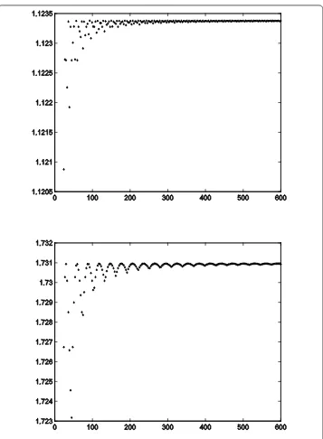
Figure 1The spectral radius ofMMTandMMT, respectively (from top to bottom)

h1≈[–0.0047182543, –0.0021152562, 0.0030907400, 0.038680809, 0.033766352,

0.016128444, –0.75722871, 1.3447918],

h2≈[0.14107656, 0.063246501, –0.092413623, –0.45441064, –0.69483538,

–0.94219467, 4.8815912, 0]/4

(12)

[image:12.595.116.479.79.330.2]

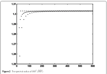
Figure 2The spectral radius ofMMT(MMT)

is an approximation and not an exact value. Similarly,T–1_≈_{1.32. By Theorem 2.5, we} can calculate that 0.66≤ T ≤1.15 and 0.94≤ T–1_≤_1.51.

Example 3.2 In [20], a 4-band symmetric biorthogonal wavelets which is denoted as Op(12-12) is designed. The corresponding wavelet ﬁlter banks{h,g1_,_g2_,_g3_}_{are as follows:}

⎡ ⎢ ⎢ ⎢ ⎣

t0 t1 t2 t3 t4 t5 t5 t4 t3 t2 t1 t0 t1 –t0 –t3 t2 t5 –t4 –t4 t5 t2 –t3 –t0 t1 t0 –t1 t2 –t3 t4 –t5 t5 –t4 t3 –t2 t1 –t0 t1 t0 –t3 –t2 t5 t4 –t4 –t5 t2 t3 –t0 –t1

⎤ ⎥ ⎥ ⎥ ⎦,

where t0 = 0.01129264, t1 = –0.01660958, t2 = –0.01418315, t3 = 0.02102888, t4 = 0.4676785, t5 = 0.5307927,t0 = –0.07653,t1 = –0.04528,t2 = 0.01722,t3 = 0.11097, t4= 0.46556,t5= 0.52806.

It has been shown that the eigenvalues ofMT

4nM4nappear in pairs of reciprocal,M4TnM4n andMT

4nM4 nhave the same eigenvalues [20]. It is obvious thatmax{λi}=max{λi}=min1{λi}=

1

min{λi}. See Fig. 2 for the spectral radius ofMnM

T

n andMnMTn. From Theorem 2.3, we can obtainT ≈1.14, which is an approximation and not an exact value. According to Theorem 2.5, we haveT=T–1_≤_1.18.

4 Conclusions and future work

(13)

Acknowledgements

The authors would like to thank the editors and reviewers for their valuable comments, which greatly improved the readability of this paper. This work supported by the Natural Science Foundation of Hunan Province (No. 16JJ6102), the Outstanding Youth Foundation of Hunan Province Department of Education (No. 17B182), the Doctoral Foundation of Hunan University of Arts and Science (No. 15BSQD02), the College Students Research Study and Innovative Experiment Project of Hunan Province (No. 17541).

Competing interests

The authors declare that they have no competing interests.

Authors’ contributions

All authors contributed to each part of this work equally and read and approved the ﬁnal manuscript.

Author details

1_{Hunan Province Cooperative Innovation Center for The Construction Development of Dongting Lake Ecological}

Economic Zone, Hunan University of Arts and Science, Changde, P.R. China.2_{College of Mathematics and Computer}

Science, Hunan Normal University, Changsha, P.R. China.

Publisher’s Note

Springer Nature remains neutral with regard to jurisdictional claims in published maps and institutional aﬃliations.

Received: 11 October 2017 Accepted: 3 February 2018

References

1. Daubechies, I., Han, B., Ron, A., Shen, Z.: Framelets, MRA-based constructions of wavelet frames. Appl. Comput. Harmon. Anal.14, 1–46 (2003)

2. Gavruta, L.: Frames for operators. Appl. Comput. Harmon. Anal.32, 139–144 (2012)

3. Sun, W., Zhou, X.: Density and stability of wavelet frames. Appl. Comput. Harmon. Anal.15, 117–133 (2003) 4. Heil, C., Kutyniok, G.: Density of wavelet frames. J. Geom. Anal.13, 479–493 (2003)

5. Kim, H., Kim, R., Lee, Y., Yoon, J.: Quasi-interpolatory reﬁnable functions and construction of biorthogonal wavelet systems. Adv. Comput. Math.33, 255–283 (2010)

6. Cohen, A., Daubechies, I., Feauveau, J.: Biorthogonal bases of compactly supported wavelets. Commun. Pure Appl. Math.45, 485–560 (1992)

7. Didenko, V.: Spectral radii of reﬁnement and subdivision operators. Proc. Am. Math. Soc.33, 2335–2346 (2005) 8. Han, B.: Symmetric orthonormal scaling functions and wavelets with dilation factor 4. Adv. Comput. Math.8, 221–247

(1998)

9. Bi, N., Dai, X., Sun, Q.: Construction of compactly supported M-band wavelets. Appl. Comput. Harmon. Anal.6, 113–131 (1999)

10. Chui, C., Lian, J.: Construction of compactly supported symmetric and antisymmetric orthonormal wavelets with scale = 3. Appl. Comput. Harmon. Anal.2, 68–84 (1995)

11. Zou, Q., Wang, G., Yang, M.: Spectral radius of biorthogonal wavelets with its application. J. Korean Math. Soc.51, 941–953 (2014)

12. Wang, G., Zou, Q., Yang, M.: Sub-band operators and saddle point wavelets. Appl. Math. Comput.227, 27–42 (2014) 13. Cui, L., Zhai, B., Zhang, T.: Existence and design of biorthogonal matrix-valued wavelets. Nonlinear Anal., Real World

Appl.10, 2679–2687 (2009)

14. Jiang, Q.: Biorthogonal wavelets with 4-fold axial symmetry for quadrilateral surface multiresolution processing. Adv. Comput. Math.34, 127–165 (2011)

15. He, T.: Biorthogonal wavelets with certain regularities. Appl. Comput. Harmon. Anal.11, 227–242 (2001) 16. Zhuang, X.: Matrix extension with symmetry and construction of biorthogonal multiwavelets with any integer

dilation. Appl. Comput. Harmon. Anal.33, 159–181 (2012)

17. Chui, C., Shi, X.: Inequalities of Littlewood–Paley type for frames and wavelets. SIAM J. Math. Anal.24, 263–277 (1993) 18. Naylor, A., Sell, G.: Linear Operator Theory in Engineering and Science. Springer, New York (2000)

19. Wang, G.: Four-bank compactly supported bi-symmetric orthonormal wavelets bases. Opt. Eng.43, 2362–2368 (2004)

20. Zou, Q., Wang, G.: Optimal model for 4-band biorthogonal wavelets bases for fast calculation. J. Inequal. Appl.2017, Article ID 222 (2017)