Exponential Stability of Time Switched Two Subsystem Nonlinear Systems with Application to Intermittent Control

Volume 2009, Article ID 348242,23pages doi:10.1155/2009/348242

Research Article

Exponential Stability of Time-Switched

Two-Subsystem Nonlinear Systems with

Application to Intermittent Control

Chuandong Li

_{and Tingwen Huang}

1_{College of Computer, Chongqing University, Chongqing 400030, China}

2_{Science Program, Texas A&M University at Qatar, P.O. Box 23874, Doha, Qatar}

Correspondence should be addressed to Tingwen Huang,[email protected] Received 15 February 2009; Revised 9 July 2009; Accepted 16 September 2009

Recommended by Kok Teo

This paper studies the exponential stability of a class of periodically time-switched nonlinear systems. Three cases of such systems which are composed, respectively, of a pair of unstable subsystems, of both stable and unstable subsystems, and of a pair of stable systems, are considered. For the first case, the proposed result shows that there exists periodically switching rule guaranteeing the exponential stability of the whole system withsufficientsmall switching period if there is a Hurwitz linear convex combination of two uncertain linear systems derived from two subsystems by certain linearization. For the second case, we present two general switching criteria by means of multiple and single Lyapunov function, respectively. We also investigate the stability issue of the third case, and the switching criteria of exponential stability are proposed. The present results for the second case are further applied to the periodically intermittent control. Several numerical examples are also given to show the effectiveness of theoretical results. Copyrightq2009 C. Li and T. Huang. This is an open access article distributed under the Creative Commons Attribution License, which permits unrestricted use, distribution, and reproduction in any medium, provided the original work is properly cited.

1. Introduction

In the recent years, motivated by the fact that many practical systems are inherently multimodal in the sense of that several dynamical systems are required to describe their behavior which may depend on various environmental factors1,2, and by the fact that the

methods of intelligent control design are based on switching between different controllers 2, 3, the study of switched systems has been received an increasing attention in control

theory and applications2,4–13. It is also worth noting that the switching rule is naturally

have been characterized in 4–7, and the switched control synthesis designs have been

presented in 2,8,9. For the time-switched systems, we refer the readers to14–16. One

can see that the study of time-switched systems is almost limited to the linear subsystems, at most with the nonlinear perturbations. In14, the switched system consists of only Hurwitz

stable subsystems. The papers15,16deal with the switched systems with both stable and unstable subsystems by means of average dwell time approach.

In the present paper, we study the exponential stability of time-periodically switched systems composed of a pair of nonlinear subsystems with neural-type Lipstchiz nonlinearities i.e., the nonlinear vector-valued function fx is of the form fx

f1x1, f2x2, . . . , fnxnT. Three cases of such systems will be dealt with.

Case 1. Periodically switched system with a pair of unstable nonlinear subsystems.

Case 2. Periodically switched system with both stable and unstable nonlinear subsystems.

Case 3. Periodically switched system with a pair of stable nonlinear subsystems.

For the first case, a linearization transformation is introduced to shift the exponential stability issue of the original system into the robustly exponential stability of the transformed system with a pair of linear time-varying subsystems, and we will use the average-system approach to analyze the robustly exponential stability of the transformed systems. For the second and third cases, the general theoretical frameworks based on the multiple Lyapunov functions will be established. We also suggest that if there exists a common Lyapunov function Vx such thati for the second case, ˙Vx ≤ −λ1Vx for the first subsystem and ˙Vx ≤ λ2Vxfor the second subsystem, then the system as a whole will be globally exponentially stable for any switching period T and any switching rate α satisfying 1 > α > λ2/λ1 λ2; iifor the third case, ˙Vx ≤ −λiVx, i 1,2, for theith subsystem, then the system as a whole will be globally exponentially stable for any switching period

T and any switching rate αsatisfying 1 > α > 0. Note also that for the first case because both subsystems are unstable there is no such common Lyapunov functionVxthat ˙Vx

is negative definite for any subsystem. Based on the stability analysis of the second case, we address the periodically intermittent output feedback control problem. Several numerical examples will be presented to show the validity of the theoretical results.

The rest of the paper is organized as follows. In the next section, the problem to be dealt with is formulated and the necessary preliminaries are presented. Then, the theoretical results for three cases of time-switched systems are established in Sections3–5, respectively.

Section 6deals with the stabilization problem by means of periodically intermittent control. InSection 7, several examples are given to verify the effectiveness of the theoretical results.

Finally, conclusions are drawn inSection 8.

2. Problem Formulation and Preliminaries

Consider a class of periodically time-switched systems withmsubsystems

˙

xt Aixt Bifixt, kT τi−1≤t < kT τi,

wherex∈Rn_{denotes the state vector,A}

i a_kli∈Rn×nandBi b_kli∈Rn×n, i1,2, . . . , m, are all constant matrices,T >0 is called the switching period,Δτiτi−τi−1is called the time duration of theith subsystem with 0 τ0 < τ1 < · · · < τm−1 < τm T. It is clear that the system2.1is a class of periodically time-switched systems withmnonlinear subsystems. Throughout this paper, we also assume thatfix fi1x1, fi2x2, . . . , finxnTwithfi0 0 are continuous functions satisfying the following condition.

H1There exist constant scalar numbersαij i1,2, . . . , m; j1,2, . . . , nsuch that

fij

y≤αijy, for anyy∈R. 2.2

In order to linearize system2.1, we definem×nfunctionssij i1,2, . . . , m;j1,2, . . . , n as follows:

sijt:

⎧ ⎪ ⎨ ⎪ ⎩

fij

xjt

xjt

, xjt/0,

0, xjt 0.

2.3

LetSidiagsi1, si2, . . . , sin, i1,2, . . . , m. Then, system2.1can be rewritten as

˙

xt Ai BiSitxt, kT τi−1≤t < kT τi,

i1,2, . . . , m, k1,2, . . . . 2.4

Notice that assumptionH1implies that|sij| ≤αij i1,2, . . . , m; j1,2, . . . , n. Therefore, we have, for anyt≥t0andi1,2, . . . , m,

−Li≤Si≤Lidiagαi1, αi2, . . . , αin. 2.5

Furthermore, let, fori1,2, . . . , m, be

|Bi| b_kli

n×n, Ci c

i kl

n×n≡Ai− |Bi|Li, Ci c

i kl

n×n≡Ai |Bi|Li,

MC_i, Ci

C c_kli

n×n:c

i kl ≤c

i

kl ≤c

i

kl, k, l1,2, . . . , n

.

2.6

Then, for anyt≥t0, we have

Ai BiSit∈M

C_i, Ci

In order to formulate the transformation, we still need the following quantities:

Ci

C_i Ci

2 A1, Hi

Ci−C_i

2 |Bi|Li, i1,2, . . . , m. 2.8

Because the entries of matrixHi h_kli∈Rn×n i1,2, . . . , mare nonnegative, we further define Ei ⎡ ⎢ ⎢ ⎢ ⎢ ⎢ ⎢ ⎢ ⎢ ⎢ ⎣

h₁₁i · · ·

h₁i_n 0 · · · 0 · · · 0 · · · 0

0 · · · 0

h₂₁i · · ·

h₂i_n · · · 0 · · · 0

· · · . .. · · · ·

0 · · · 0 0 · · · 0 · · ·

h_ni₁ · · ·

hnni

⎤ ⎥ ⎥ ⎥ ⎥ ⎥ ⎥ ⎥ ⎥ ⎥ ⎦ , Fi ⎡ ⎢ ⎢ ⎢ ⎢ ⎢ ⎢ ⎢ ⎢ ⎢ ⎢ ⎢ ⎢ ⎢ ⎢ ⎢ ⎢ ⎢ ⎢ ⎢ ⎢ ⎢ ⎢ ⎢ ⎢ ⎢ ⎢ ⎢ ⎢ ⎢ ⎢ ⎢ ⎣

h₁₁i · · · 0

· · · . .. · · ·

0 · · ·

h₁i_n

h₂₁i· · · 0

· · · . .. · · ·

0 · · ·

h₂i_n

· · · ·

h_ni₁ · · · 0

· · · . .. · · ·

0 · · ·

hnni

⎤ ⎥ ⎥ ⎥ ⎥ ⎥ ⎥ ⎥ ⎥ ⎥ ⎥ ⎥ ⎥ ⎥ ⎥ ⎥ ⎥ ⎥ ⎥ ⎥ ⎥ ⎥ ⎥ ⎥ ⎥ ⎥ ⎥ ⎥ ⎥ ⎥ ⎥ ⎥ ⎦ . 2.9

Simple computation yields, fori1,2, . . . , m,

EiETi diag

⎛

⎝n

j1

h₁i_j,

n

j1

h₂i_j, . . . ,

n

j1

h_nji

⎞

⎠_,

FT_iFidiag

⎛

⎝n

j1

h_ji₁,

n

j1

h_ji₂, . . . ,

n

j1

h_jni

⎞

⎠_.

2.10

Lemma 2.1See17,18. Let

Σ∗_Σ∈Rn2_×n2

|Σ diagε11, . . . , ε1n, . . . , εn1, . . . , εnn, εij≤1, fori, j1,2, . . . , n

,

NC_i, Ci

{DiCi EiΣiFi|Σi∈Σ∗}.

2.11

Then,MC_i, Ci NC_i, Ci.

Proof. A proof of this lemma is presented in the appendix.

Now, we consider the following uncertain linear system withΣi∈Σ∗, i1,2,

˙

xt Ci EiΣiFixt, kT τi−1≤t < kT τi. 2.12

It follows fromLemma 2.1that the parameter uncertainties in2.4and2.12are identical, which implies that 2.12is equivalent to system 2.4. It is also observed that the robust

stability property of2.4implies the stability property of system2.1. Therefore, in order to

derive the sufficient conditions for stability of system2.1, we consider the robust stability

of system2.12.

Remark 2.2. If the nonlinear functionfixsatisfies the assumption

H2forxj/0 andi1,2, . . . , m; j 1,2, . . . , n, 0≤fijxj/xj≤αij.

Then, 0≤sij≤αijandCiAi min{0, b_kliαil}, Ci Ai max{0, b_kliαil}. This implies that

CiAi 1/2b_kliαil, Hi 1/2|b_kli|αil, wheredkldenotes a matrix withdklas thekth line andlth column entry.

For briefness, we mainly focus on system2.1with two subsystems in the sequel, that is,m2. In this case, we rewrite, respectively, systems2.1and2.12as

˙

xt A1xt B1fxt, kT ≤t < kT αT,

˙

xt A2xt B2gxt, kT αT≤t <k 1T,

2.13

˙

xt C1 E1Σ1F1xt, kT≤t < kT αT,

˙

xt C2 E2Σ2F2xt, kT αT ≤t <k 1T,

2.14

where 0 < α < 1 is called the switching rate. The results for2.13and/or2.14are easily extended to the general systems2.1and/or2.12withmsubsystems.

The following two lemmas are useful in the sequel.

Lemma 2.3Sanchez and Perez19. Given any real matricesΣ1,Σ2,Σ3of appropriate dimensions

and a scalarε >0such that0<Σ3 ΣT₃. Then, the following inequality holds:

ΣT

1Σ2 ΣT2Σ1≤εΣT1Σ3Σ1 ε−1ΣT2Σ−31Σ2, 2.15

Lemma 2.4Schur complement, Boyd et al.20. The following LMI:

Qx Sx

ST_{x Rx}

>0, 2.16

whereQx QT_{x,Rx R}T_{x, andSxdepend affinely onx, is equivalent to}

Rx>0, Qx−SxR−1_xST_{x>0. 2.17}

Throughout this paper, we denote by PT the transpose of matrix P; λminP and

λmaxP the minimal and maximal eigenvalues of a real symmetric matrixP, respectively;

P >0≥, <,≤0the symmetrical and positivesemipositive, negative, seminegativedefinite matrixP, andPthe Euclidian norm of the square matrix.

3. Stability Analysis for the First Case

In this section, we consider system2.13 composed of a pair of unstable subsystems with neural-type nonlinearities. Since the robust stability property of system 2.14 implies the stability property of the original system 2.13, we will derive a sufficient condition of

globally exponential stability. The theoretical result shows that similar switching criterion guaranteeing the exponential stability of the origin of time-switched LTI systems still holds for time-switched nonlinear systems with neural-type nonlinearities.

The main result in this section is as follows.

Theorem 3.1. Suppose that there exist symmetric and positive definite matrixP, positive constants

q1, q2, andα0< α <1such that

Ω1PαC1 1−αC2 αC1 1−αC2TP αq₁−1P E1ET₁P αq1F₁TF1

1−αq−1

2 P E2ET2P 1−αq2F2TF2<0,

3.1

whereCi, Ei, and Fii1,2are defined, respectively, in2.8. Then, there exists (small) switching

period T such that the origin of time-switched system2.14is globally robustly exponentially stable,

and therefore system2.13is globally exponentially stable.

Proof. We only need to show that inequality3.1implies the robustly exponential stability

initial value isx0 xt0with the starting timet0 ∈0, αT. Then, by piecewise integration, we have

xαT expC1 E1Σ1F1αT−t0x0,

xT expC2 E2Σ2F21−αTexpC1 E1Σ1F1αT−t0x0

expC2 E2Σ2F21−αTexpC1 E1Σ1F1αTexp−C1 E1Σ1F1t0x0

I C2 E2Σ2F21−αT 1

2!C2 E2Σ2F2

2_1−α2_T2 _{· · ·}

×

I C1 E1Σ1F1αT 1

2!C1 E1Σ1F1

2_α2_T2 _{· · ·}

×exp−C1 E1Σ1F1t0x0

{I C1 E1Σ1F1α C2 E2Σ2F21−αT OT} ×exp−C1 E1Σ1F1t0x0.

3.2

Along this idea and omitting the termsOTwhenTtends to zero, one observes that if we let

Ttend to zero, on any fixed time interval the solution of2.14will tend to the solutionwith the same initial conditionof the following “averaged” systemsee21for more details, for

anyΣ1, Σ2 ∈Σ∗,

˙

xt C1 E1Σ1F1α C2 E2Σ2F21−αxt. 3.3

In particular, the stability properties of the switched system2.14will for sufficiently small

T be determined by the robust stability properties of the averaged system3.3. Note that

system3.3is globally exponentially stable if and only if there exists 0 < α < 1 such that

Ae C1 E1Σ1F1α C2 E2Σ2F21−αis Hurwitz for anyΣ1, Σ2∈Σ∗, which is equivalent to the fact that there exists symmetric and positive definite matrixPsuch thatAT

eP P Ae<0. A sufficient condition for this inequality is justΩ1<0, that is, inequality3.1. This is because, forx /0,

xTAT_eP P Ae

xxTC1 E1Σ1F1α C2 E2Σ2F21−αTP

PC1 E1Σ1F1α C2 E2Σ2F21−α

x

xTαC1 1−αC2TP PαC1 1−αC2

x

2αxTP E1Σ1Fx 21−αxTP E2Σ2F2x

≤xTαC1 1−αC2TP PαC1 1−αC2

x αq₁−1xTP E1E1TP x

αq1xTF1TF1x 1−αq2−1xTP E2E

T

xT_αC

1 1−αC2TP PαC1 1−αC2 αq1−1P E1ET1P αq1F1TF1

1−αq₂−1P E2E2TP 1−αq2F2TF2

x

xTΩ1x <0.

3.4

This concludes the proof.

Remark 3.2. This result is seen as the natural extension of that of time-switched linear systems

16.

4. Stability Analysis for the Second Case

In this section, we consider system2.13composed of both stable and unstable subsystems with neural-type nonlinearities. By means of, respectively, multiple and single Lyapunov function, we propose two general criteria, together with simple but effective sufficient conditions guaranteeing the globally exponential stability.

Reconsider the time-switched system2.13. Here we assume that the first subsystem

is globally exponentially stable at the origin, while the second one unstable. It is natural that the system as a whole will be globally exponentially stable for any given 0 < α < 1 when the switching periodTapproaches to infinite andt0 ∈kT, kT αT. Our interest here is to determine a region of the binaryT, αcomposed of the switching periodT and switching rateαsuch that the system as a whole is globally exponentially stable therein.

Theorem 4.1. Suppose that there exist two scalar functionsVi : Rn → R , i 1,2, a continuous

and monotonously increasing functionγwithγ0 0and constantsλ1 >0,λ2 >0andβ≥1such

that the following conditions hold:

iγx≤V1x;

iifor anyk 0,1,2, . . ., whent∈kT, kT αT,V˙1x≤ −λ1V1x, and whent∈kT

αT,k 1T,V˙2x≤λ2V2x;

iiiVix≤βVjx, for anyx∈Rnandi, j∈ {1, 2}; ivεαλ1−1−αλ2−2/Tlnβ >0.

Then, the origin of the time-switched system2.13is globally exponentially stable.

Proof. Whent∈kT, kT αT, it follows from conditioniithat

V1x≤exp{−λ1t−kT}V1kT. 4.1

Similarly, whent∈kT αT,k 1T, the differential inequality ˙V2x≤λ2Vximplies

From4.1-4.2and conditioniii, we have the following

aWhent∈0, αT,V1x≤exp{−λ1t}V10. bWhent∈αT, T,

V2x≤exp{λ2t−αT}V2αT

≤βexp{λ2t−αT}V1αT ≤βexp{λ2t−αT−λ1αT}V10 βexp{−λ1 λ2αT λ2t}V10.

4.3

cWhent∈T, T αT,

V1x≤exp{−λ1t−T}V1T

≤βexp{−λ1t−T}V2T

≤β2exp{−λ1t−T−λ1 λ2αT λ2T}V10

β2exp{λ1 λ21−αT−λ1t}V10.

4.4

dWhent∈T αT,2T,

V2x≤exp{λ2t−T−αT}V2T αT

≤βexp{λ2t−T−αT}V1T αT

≤β3exp{λ2t−T−αT λ1 λ21−αT−λ1T αT}V10

β3_exp{−2λ

1 λ2αT λ2t}V10.

4.5

By induction, we have the following.

eWhent∈kT, kT αTwhich impliesk≤t/T,

V1x≤β2kexp{kλ1 λ21−αT −λ1t}V10

≤exp λ1 λ21−αT 2 lnβ

!t T −λ1t

"

V10

≤exp

λ1 λ21−α 2

T lnβ

t

"

V10

exp

−

αλ1−1−αλ2− 2

T lnβ−λ1

t

"

V10.

fWhent∈kT αT,k 1Twhich impliesk 1≥t/T≥k,

V2x≤β2k 1exp{−k 1λ1 λ2αT λ2t}V10

≤βexp −λ1 λ2αT 2 lnβ

!t T λ2t

"

V10

≤βexp

−

λ1 λ2α− 2

T lnβ−λ2

t

"

V10

βexp

−

αλ1−1−αλ2− 2

T lnβ

t

"

V10.

4.7

Therefore, we can conclude the proof frome-fand conditionsiandiv.

Based on Theorem 4.1, if we choose the quadratic Lyapunov function Vix

xT_P

ix2 i1,2for theith subsystem, the following result is immediate.

Corollary 4.2. Suppose that there exist symmetric and positive definite matrices P1 and P2, the

positive constantsλ1, λ2, μ1,andμ2such that

iP1A1 0.5λ1I A1 0.5λ1ITP1 μ−₁1P1B1B₁TP1 μ1L2₁≤0, iiP2A2−0.5λ2I A2−0.5λ2ITP2 μ−₂1P2B2BT₂P2 μ2L2₂≤0, iiiεαλ1−1−αλ2−2/Tlnβ >0,

where β sup_{1≤i /j≤2}λmaxPi/λminPj. Then, by the switching period T with switching rate

α, the origin of time-switched system2.13 with both stable and unstable subsystems is globally

exponentially stable. Moreover, the norm of state vector satisfies the following inequality:

xt ≤

#

βλmaxP1

λminP1

x0exp

−1 2

αλ1−1−αλ2− 2

T lnβ

t

"

. 4.8

Proof. Consider the Lyapunov functionVix xTPixi1, 2. Whent∈kT, kT αT, from

conditioniandLemma 2.3the derivative ofV1along the trajectories of the first subsystem is calculated and estimated as follows:

˙

V1x 2xTP1 A1xt B1fxt

!

xTtP1A1 AT₁P1

xt 2xTtP1B1fxt

≤xTtP1A1 AT₁P1

xt μ−₁1xTtP1B1B₁TP1xt μ1fTxtfxt

≤xTtP1A1 AT1P1 μ−11P1B1BT1P1

xt μ1xTtL21xt

xTtP1A1 AT1P1 μ1−1P1B1BT1P1 μ1L21

xt

−λ1V1x xTt

P1A1 AT1P1 μ−11P1B1B1TP1 μ1L21 λ1P1

xt

≤ −λ1V1x.

Similarly, based on conditioniiandLemma 2.3, fort∈kT αT,k 1T, we have

˙

V2x 2xTP2 A2xt B2gxt

!

xTtP2A2 AT2P2

xt 2xTtP2B2gxt

≤xTtP2A2 AT2P2

xt μ−₂1xTtP2B2BT2P2xt μ2gTxtgxt

≤xTtP2A2 AT₂P2 μ−₂1P2B2BT₂P2

xt μ2xTtL2₂xt

xTtP2A2 AT2P2 μ2−1P2B2BT2P2 μ2L22

xt

λ2V2x xTt

P2A2 AT2P2 μ−21P2B2B2TP2 μ2L22−λ2P2

xt

≤λ2V2x.

4.10

Therefore, conditions i-ii in Theorem 4.1 hold. Obviously, the definition of β implies

Vix≤βVjxwhich leads to conditioniiiinTheorem 4.1. Thus, we complete the proof.

Remark 4.3. ConditionivinTheorem 4.1and conditioniiiinCorollary 4.2hold for large

enough switching periodTifαλ1−1−αλ2>0. This is completely consistent with the extreme case that only the stable system is activated, that is,T ∞.

Remark 4.4. Conditioniiiin this theorem can help to derive an estimated regionΩof period

Tand switching rateα, where each binaryα, T∈Ωcan guarantee the exponential stability of system2.13. For computational consideration, we suggest the following steps.

aFind the maximum λ1 and the corresponding P1 from condition i which is equivalent to the following linear matrix inequality with respect toP1andμ1this follows fromLemma 2.4:

P1A1 AT₁P λ1P μ1L2₁ −P B1 −BT₁P −μ1I

≤0. 4.11

bTherefore, this step is changed into solving the optimization problem

maxλ1

s.t.,

P1A1 AT₁P λ1P μ1L2₁ −P B1 −BT

1P −μ1I

cFind the minimumλ2and the correspondingP2from conditioniiby solving the optimization problem

minλ2

s.t.,

P2A2 AT₂P2 μ2L2₂−λ2P2 −P2B2 −BT

2P2 −μ2I

≤0. 4.13

dEstimate the region ofα, T

Ω

α, T : αλ1−1−αλ2>0, T >

2 lnβ αλ1−1−αλ2

"

. 4.14

Then, for anyα, T∈Ω, system2.13is globally exponentially stable.

Similarly, following the idea of the proof ofTheorem 4.1, we have the simpler result when a common Lyapunov function is chosen.

Theorem 4.5. Suppose that there exist a Lyapunov function V : Rn _{→ R , a continuous and}

monotonously increasing functionγwithγ0 0, and constantsλ1>0,λ2>0, andβ≥1such that

the following conditions hold:

iγx≤Vx;

iifor anyk 0,1,2, . . ., whent∈ kT, kT αT,V˙x≤ −λ1Vx, and whent ∈kT

αT,k 1T,V˙x≤λ2Vx; iiiεαλ1−1−αλ2>0.

Then, the origin of the time-switched system2.13is globally exponentially stable for any switching

periodT >0.

Proof. The proof is similar with that ofTheorem 4.1, and omitted here.

From this theorem, a standard Lyapunov function Vx xTP x will yield the following corollary.

Corollary 4.6. Suppose that there exist symmetric and a positive definite matrix P, four positive

constantsλ1, λ2, μ1,andμ2such that

iPA1 0.5λ1I A1 0.5λ1ITP μ−₁1P B1B₁TP μ1L2₁≤0, iiPA2−0.5λ2I A2−0.5λ2ITP μ−₂1P B2BT₂P μ2L2₂≤0, iiiεαλ1−1−αλ2>0.

Then, for any switching period T > 0, the origin of time-switched system 2.13 is globally

exponentially stable. Moreover, the norm of state vector satisfies the following inequality:

xt ≤

#

λmaxP

λminPx0exp

−1

2αλ1−1−αλ2t

"

We now study this problem by using the linearization system2.14andTheorem 4.5. A simpler sufficient condition for exponential stability of system2.13with both stable and unstable subsystems is established.

Corollary 4.7. Suppose that there exist symmetric and positive definite matrixP, positive constants

λ1, λ2, μ1,and μ2such that

iP C1 CT1P μ−11P E1E1TP μ1F1TF1 λ1P ≤0, iiP C2 CT₂P μ−₂1P E2E₂TP μ2F₂TF2−λ2P ≤0,

then, for arbitraryT >0, if1> α > λ2/λ1 λ2, the origin of time-switched system2.13with both stable and unstable subsystems is globally exponentially stable.

Proof. Consider the common Lyapunov functionVx xT_{P xfor both subsystems. The rest}

of the proof is similar to that ofTheorem 4.1, and hence omitted.

Remark 4.8. In Corollaries4.6and4.7, conditioniis to guarantee the exponential stability of

the first subsystem, while the instability of the second subsystem follows conditionii.

Remark 4.9. For computational consideration, we suggest the following algorithm.

aFind the maximumλ1and the correspondingPfrom conditioniinCorollary 4.6 orCorollary 4.7by using the convex optimization algorithm.

bFind the minimumλ2from conditioniiinCorollary 4.6orCorollary 4.7by using the convex optimization algorithm. Note that the matrixP is solved ina.

cCalculate the low bound ofα,λ2/λ1 λ2. Then, for anyT >0, if 1> α > λ2/λ1 λ2, system2.13is globally exponentially stable.

5. Stability Analysis for the Third Case

In this section, we consider the time-switched system2.13with a pair of stable subsystems. The contribution is twofold. Firstly, for the linear case, we characterize the stability properties in four aspects. Secondly, we extend the results for the linear case to the nonlinear system with neural-type nonlinearities.

5.1. Linear Case

Consider the following time-switched system with a pair of stable linear subsystems:

˙

xt A1xt, kT ≤t < kT αT,

˙

xt A2xt, kT αT≤t <k 1T,

x0 x0,

5.1

wherex∈Rn_{denotes the state vector,A}

Theorem 5.1. System5.1with a pair of stable subsystems is globally exponentially stable for any switching rule if there exists a symmetric and positive definite matrix P such that both the following inequalities hold:

iP A1 AT₁P <0, iiP A2 AT2P <0.

Proof. Consider the common Lyapunov functionVx xT_{P x. Integrating by partVxwith}

respect to timetalong the trajectories of the system5.1, we have, for anyt >0,

Vx≤KxT₀P x0exp{−αλ1 1−αλ2t}, 5.2

whereK exp{α1−αλ2T}, and λi is positive constant and satisfies P Ai ATiP λiP < 0, i1,2. Note that for any 0< α <1, αλ1 1−αλ2 >0, and therefore,5.2concludes the proof.

When the condition inTheorem 5.1does not hold, we suggest the following claim.

Theorem 5.2. Let

λi sup PPT_>0

λ:P Ai ATiP λP <0, λ >0

, _5.3

Piarg

$

sup PPT_>0

λ:P Ai ATiP λP <0, λ >0

%

, i1,2. 5.4

Then, system5.1is globally exponentially stable if the switching period T satisfies

T > 2 lnβ αλ1 1−αλ2

, 5.5

whereβmax1≤i /j≤2{λmaxPi/λminPj}.

Proof. Consider the multiple Lyapunov function

V1x xTP1x, t∈kT, kT αT,

V2x xTP2x, t∈kT αT,k 1T.

5.6

Note thatPiAi AT_iPi λiPi≤0. We calculate the derivatives ofViwith respect to timetalong the trajectories of the system5.1as follows:

˙

Therefore, we have

afor anyt∈kT, kT αT,

Vx≤V10exp

−

αλ1 1−αλ2− 2 lnβ

T

kT

"

, 5.8

bfor anyt∈kT αT,k 1T,

Vx≤βexp{−αλ1T}V10exp

−

αλ1 1−αλ2− 2 lnβ

T

kT

"

. 5.9

Hence, ifαλ1 1−αλ2−2 lnβ/T >0, that is,T >2 lnβ/αλ1 1−αλ2, system5.1is globally exponentially stable. The proof is thus completed.

5.2. Nonlinear Case

Consider again the nonlinear time-switched system 2.13 and the “linearization” system 2.14, but in this section we assume that both subsystems in2.14are robust Hurwitz-stable. Arguing similarly with the previous subsection, we have the analogs of the results described by Theorems5.1and5.2.

Theorem 5.3. Assume that, fori1,2,

λi sup PPT_>0

Σi∈Σ∗

λ:PCi EiΣiFi Ci EiΣiFiTP λP <0, λ >0

,

Piarg

⎛ ⎜

⎝ sup

PPT_>0 Σi∈Σ∗

λ:PCi EiΣiFi Ci EiΣiFiTP λP <0, λ >0

⎞_⎟

⎠,

5.10

exist. Then, the origin of system2.13is globally exponentially stable if any one of the following

conditions holds.

iThere exists a symmetric and positive definite matrix P such that

PCi EiΣiFi Ci EiΣiFiTP <0, i1,2, 5.11

is satisfied for anyΣi∈Σ∗.

iiThe switching period T satisfies

T > 2 lnβ αλ1 1−αλ2

, 5.12

Notice that, for anyμi>0,

PCi EiΣiFi Ci EiΣiFiTP ≤P Ci CiTP μ−i1P EiEiTP μiFiTFi. 5.13

Then, the following corollary is immediate.

Corollary 5.4. System2.13is globally exponentially stable if any one of the following conditions

holds.

iThere exist a symmetric and positive definite matrix P and positive constantsμisuch that

P Ci CiTP μi−1P EiETiP μiFiTFi<0, i1,2, hold. 5.14

iiIf, fori1,2, there exist symmetric and positive definite matricesPiand positive constants

λisatisfying

λi sup PPT_>0

μi>0

λ:P Ci CT_iP μ−_i1P EiET_iP μiF_iTFi λP <0, λ >0

,

Piarg

⎛ ⎜

⎝ sup

PPT_>0

μi>0

λ:P Ci CTiP μ−i1P EiETiP μiFiTFi λP <0, λ >0

⎞_⎟

⎠,

5.15

and further the switching periodTand switching rateαsatisfyT >2 lnβ/αλ1 1−αλ2, where

βmax1≤i /j≤2{λmaxPi/λminPj}.

6. Intermittent Control with Time Duration

scheme to decouple neighboring qubits in quantum computers through bang-bang pulse control and demonstrated that two similar sequence of pulses with different time intervals not only suppress decoherence but entirely or selectively decouple two neighboring qubits. The authors in27–31suggested to controlling the evolution of a system by using strong, short pulses as a new means for quantum error prevention. Also, the authors in32discussed chaotic synchronization by using intermittent control.

An extreme case of intermittent control is impulsive control which has been gained increasing interest and intensively researched 33, 34. The prominent characteristic of

impulsive control is that the states of controlled system will “jump” at certain discrete time moments, namely, the control is with zero duration of time. Because the states of controlled systems are changed directly, impulsive control is an effective approach when the states are observable, but it seems to be invalid when the states of controlled systems are unobservable. Our interest focuses on the class of intermittent control with time duration, namely, the control is activated in certain nonzero time intervals, and offin other time intervals. Specifically, the control law is of the form

ut

⎧ ⎨ ⎩

u1t, t∈tk, tk τ,

0, t∈tk τ, tk 1.

6.1

Consider the nonlinear system described by

˙

xt Axt Bfxt ut,

yt Cxt,

xt0 x0,

6.2

wherex x1, x2, . . . , xnT ∈Rndenotes the state vector,A aij∈Rn×nandB bij∈Rn×n are constant matrices, and the nonlinear function,fx f1x1, . . . , fnxnT : Rn → Rn, is continuous withf0 0, and satisfies the Lipstchitz condition with the Liptchiz constant

αi, namely,|fixi| ≤ αi|xi|, i 1,2, . . . , n.yt presents the output of the system with the coefficient matrixC cij∈Rm×n, andutis the external input with the form of6.1. For analytical simplification, we assume in this paper the inpututis periodical switching with the fixed duration of time. Specifically, we takeut, in the sequel, as the form

ut ktyt, 6.3

with

kt

⎧ ⎨ ⎩

Kn×m, 0≤t < αT,

0, αT≤t < T, 0< α <1,

kt T kt.

6.4

Note that the controlled system6.2with6.3-6.4can be rewritten as

˙

xt A KCxt Bfxt, t∈kT, kT αT,

˙

xt Axt Bfxt, t∈kT αT,k 1T,

xt0 x0, k0,1,2, . . . .

6.5

According to2.8, it is not difficult to obtainC1A KC,C2AandH1 H2 |B|L, where |B| |bij|_n×nandLdiagα1, . . . , αn. BecauseH1 H2 |B|L, both the equalitiesE1 E2 andF1 F2hold. For notational simplification, let us defineH≡H1H2, E≡E1 E2, and

F≡F1F2. FromCorollary 4.7, we have the following result.

Theorem 6.1. There exist a matrix Q ∈ Rn×m_{, and a symmetric, positive definite matrix P, and}

positive constantsλ1, λ2, andμsuch that

iQC CT_QT _λ

1 λ2P ≤0, iiP A AT_{P μ}−1_{P EE}T_{P μF}T_F−λ

2P ≤0, iii1> α > λ2/λ1 λ2.

Then, the origin of system6.5is exponentially stable for anyT >0, and the corresponding control

gain matrix is determined byKP−1_Q.

Proof. We only need to show that the conditions inCorollary 4.7 are satisfied. The proof is

trivial, and therefore omitted here.

To end this section, we consider a special external input of the formut ktyt

where

kt

⎧ ⎨ ⎩

k0, t∈kt, kT αT,

0, t∈kt αT,k 1T, k1,2, . . . , 6.6

in whichk0is a constant scalar. Then, fromTheorem 6.1, the following corollary is immediate.

Corollary 6.2. Letλ0 infμ>0{λmaxA AT μ−1EET μFTF}, andλc λmaxC CT. The

origin of controlled system6.5is exponentially stable for anyT >0if1> α >−λ0/λck0.

7. Illustrating Examples

In this section, we will give two examples to show the validity of the proposed results.

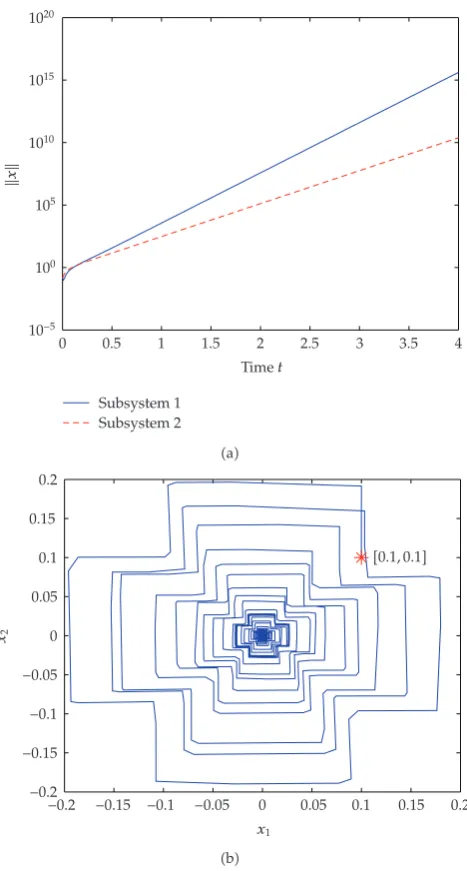
Example 7.1. Consider system2.13with

A1

−0.5 1 100 −1

, A2

−1 −100 −0.5 −1

, B1B2

−1 0 0 −1

,

fx gx

1

2|x1 1| − |x1−1|,0

T

.

Both subsystems are unstable, as shown inFigure 1a. Note that

C1

−1 1 100 −2

, C2

−1.5 −100 −0.5 −1.5

,

E1ET1 E2ET2 F1TF1F2TF2

0.5 0 0 0.5

.

7.2

TakingP I identity matrixandq1 q2 1, we have, whenα0.5,Ω1

_{−1.5 0.25}

0.25 −2

with the eigenvalues−2.104 and −1.396. Hence, it follows fromTheorem 3.1that when α 0.5 the system in this example is globally exponentially stable for some small enoughT >0, as shown inFigure 1b.

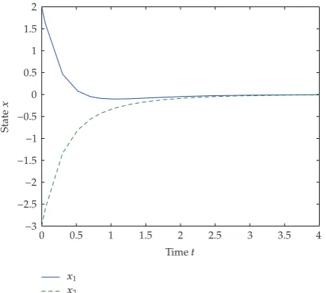
Example 7.2. Consider system2.13with

A1

−2 1 1 −2

, A2

2 2 1 3

, B1

1 0.5 −0.4 1

, B2

0.5 0 0 0.5

,

fx

1

2|x1 1| − |x1−1|,0

T

, gx

0,1

2|x1 1| − |x1−1|

T

.

7.3

Based onCorollary 4.2, solving the linear matrix inequalities by LMI ToolBox involved in the engineering software MATLAB, we obtain

λ10.3092, λ21.675 with μ117.190433, μ244.332956,

P1

11.3808 2.14237 2.14237 5.92472

, P2

39.37458 −3.427225 −3.427225 89.11437

. 7.4

Therefore,β17.235 and an estimated region ofΩis

Ω

α, t: 1.9842α−1.675−5.6939

T >0, T >0, α <1

"

, 7.5

which covers the whole region above the curve 1.9842α−1.675−5.6939/T 0 withT >0 and

α <1.

We also obtain the switching law by using Corollary 4.6. Solving condition i in

Corollary 4.6, we get the maximumλ1 0.3092 and the correspondingP; then solving the conditioniiyieldsλ2 9.8519; finally, we calculate the feasible interval of switching rate,

10−5 100 105 1010 1015 1020

x

0 0.5 1 1.5 2 2.5 3 3.5 4

Timet

Subsystem 1 Subsystem 2

a

−0.2 −0.15 −0.1 −0.05 0 0.05 0.1 0.15 0.2

x2

−0.2 −0.15 −0.1 −0.05 0 0.05 0.1 0.15 0.2

x1

0.1,0.1

b

Figure 1:aTime response curves of norm of solution vectors of two subsystems inExample 7.1.bPhase

diagram of the switched system inExample 7.1. The switching periodT 0.02, switching rateα0.5, the initial valuex0 0.1,0.1.

8. Conclusions

−3 −2.5 −2 −1.5 −1 −0.5 0 0.5 1 1.5 2

State

x

0 0.5 1 1.5 2 2.5 3 3.5 4

Timet x1

x2

Figure 2:Time response curves of states of the system inExample 7.2.

method including the “averaged” system approach, multiple and single Lyapunov function, and robust analysis of linear time-variant systems. The periodically intermittent control design problem was also addressed. This paper focuses on only the neural-type Lipstchitz nonlinearity, therefore, the further work may deal with the general nonlinear subsystems. Also, the effect of short and strong control strength on the reduction of the control cost in the presence of output noise seems to be an interesting topic.

Appendix

A Proof of

Lemma 2.1

For anyA∈NA, A, it is easy to see that there exist real constantsεij,|εij| ≤1, such that

AA0

n

i,j1

εijHij, A.1

whereHij hkl∈Rn×nsatisfies

hkl

⎧ ⎨ ⎩

h1,i,j, ki, lj,

0, otherwise. A.2

Since rankHij≤1, it can be decomposed as

Hij

h1,i,jei×

h1,i,jejT, A.3

FromA.1andA.3, we have

AA0

n

i,j1

εij×

h1,i,jei×

h1,i,jeTj. A.4

From4.1and4.2, we can see that there exists aΣA ∈Σ∗such thatAA0 EAΣAFA, that is,A ∈MA, A. Hence,NA, A⊆ MA, A. Noting that the process above is inverse, we

can also derive the relationNA, A⊇ MA, A. Therefore,NA, A MA, A. Similarly,

one can showMB, B NB, B. The proof is thus completed.

Acknowledgments

The authors are grateful to the editor and reviewers for their constructive comments based on which the presentation of the paper has been greatly improved. The work described in this paper was partially supported by the National Natural Science Foundation of China Grant no. 60974020, 10971240, the Natural Science Foundation Project of CQ CSTCGrant no. 2006BB2228and the Program for New Century Excellent Talents in University.

References

1 M. Wicks, P. Peleties, and R. Decarlo, “Switched controller synthesis for the quadratic stabilization of a pair of unstable linear systems,”European Journal of Control, vol. 4, no. 2, pp. 140–147, 1998.

2 D. Liberzon and A. S. Morse, “Basic problems in stability and design of switched systems,”IEEE Control Systems Magazine, vol. 19, no. 5, pp. 59–70, 1999.

3 A. S. Morse, “Supervisory control of families of linear set-point controllers. I. Exact matching,”IEEE Transactions on Automatic Control, vol. 41, no. 10, pp. 1413–1431, 1996.

4 M. S. Branicky, “Multiple Lyapunov functions and other analysis tools for switched and hybrid systems,”IEEE Transactions on Automatic Control, vol. 43, no. 4, pp. 475–482, 1998.

5 D. Cheng, “Stabilization of planar switched systems,”Systems & Control Letters, vol. 51, no. 2, pp. 79–88, 2004.

6 Z. G. Li, C. Y. Wen, and Y. C. Soh, “Stabilization of a class of switched systems via designing switching laws,”IEEE Transactions on Automatic Control, vol. 46, no. 4, pp. 665–670, 2001.

7 Z. Ji, L. Wang, and G. Xie, “New results on quadratic stabilization of switched linear systems with polytopic uncertainties,”IMA Journal of Mathematical Control and Information, vol. 22, no. 4, pp. 441– 452, 2005.

8 X. Xu and P. J. Antsaklis, “Stabilization of second-order LTI switched systems,”International Journal of Control, vol. 73, no. 14, pp. 1261–1279, 2000.

9 D. Liberzon, Switching in Systems and Control, Systems & Control: Foundations & Applications, Birkh¨auser, Boston, Mass, USA, 2003.

10 H. Xu, X. Liu, and K. L. Teo, “RobustH∞ stabilisation with definite attenuance of an uncertain

impulsive switched system,”The ANZIAM Journal, vol. 46, no. 4, pp. 471–484, 2005.

11 H. Xu, X. Liu, and K. L. Teo, “Delay independent stability criteria of impulsive switched systems with time-invariant delays,”Mathematical and Computer Modelling, vol. 47, no. 3-4, pp. 372–379, 2008.

12 H. Xu, X. Liu, and K. L. Teo, “A LMI approach to stability analysis and synthesis of impulsive switched systems with time delays,”Nonlinear Analysis: Hybrid Systems, vol. 2, no. 1, pp. 38–50, 2008.

13 C. Y.-F. Ho, B. W.-K. Ling, Y.-Q. Liu, P. K.-S. Tam, and K.-L. Teo, “Optimal PWM control of switched-capacitor DC-DC power converters via model transformation and enhancing control techniques,” IEEE Transactions on Circuits and Systems I, vol. 55, no. 5, pp. 1382–1391, 2008.

15 B. Hu, X. Xu, A. N. Michel, and P. J. Antsaklis, “Stability analysis for a class of nonlinear switched system,” inProceedings of the 38th IEEE Conference on Decision and Control (CDC ’99), vol. 5, pp. 4374– 4379, Phoenix, Ariz, USA, December 1999.

16 G. Zhai, B. Hu, K. Yasuda, and A. N. Michel, “Stability analysis of switched systems with stable and unstable subsystems: an average dwell time approach,” inProceedings of the American Control Conference, vol. 1, pp. 200–204, Chicago, Ill, USA, 2000.

17 C. D. Li, X. F. Liao, and R. Zhang, “Global robust asymptotical stability of multidelayed interval neural networks: an LMI approach,”Physics Letters A, vol. 328, no. 6, pp. 452–462, 2004.

18 F. X. Wu, Z. K. Shi, and Z. X. Zhou, “Robust stabilization of linear time-variant interval systems,” inProceedings of the 3rd World Conference on Intelligent Control and Automation, pp. 3415–3418, Hefei, China, July 2000.

19 E. N. Sanchez and J. P. Perez, “Input-to-state stabilityISSanalysis for dynamic neural networks,” IEEE Transactions on Circuits and Systems I, vol. 46, no. 11, pp. 1395–1398, 1999.

20 S. Boyd, L. El Ghaoui, E. Feron, and V. Balakrishnan,Linear Matrix Inequalities in System and Control Theory, vol. 15 ofSIAM Studies in Applied Mathematics, SIAM, Philadelphia, Pa, USA, 1994.

21 A. van der Schaft and H. Schumacher,An Introduction to Hybrid Dynamical Systems, vol. 251 ofLecture Notes in Control and Information Sciences, Springer, London, UK, 2000.

22 T. W. Carr and I. B. Schwartz, “Controlling unstable steady states using system parameter variation and control duration,”Physical Review E, vol. 50, no. 5, pp. 3410–3415, 1994.

23 T. W. Carr and I. B. Schwartz, “Controlling the unstable steady state in a multimode laser,”Physical Review E, vol. 51, no. 5, pp. 5109–5111, 1995.

24 T. W. Carr and I. B. Schwartz, “Controlling high-dimensional unstable steady states using delay, duration and feedback,”Physica D, vol. 96, no. 1–4, pp. 1–25, 1996.

25 J. Starrett, “Control of chaos by occasional bang-bang,”Physical Review E, vol. 67, no. 3, Article ID 036203, 4 pages, 2003.

26 T. L. Montgomery, J. W. Frey, and W. B. Norris, “Intermittent control systems for SO2,”Environmental

Science and Technology, vol. 9, no. 6, pp. 528–532, 1975.

27 Y. Zhang, Z.-W. Zhou, and G.-C. Guo, “Decoupling neighboring qubits in quantum computers through bang-bang pulse control,”Physics Letters A, vol. 327, no. 5-6, pp. 391–396, 2004.

28 L. Viola and S. Lloyd, “Dynamical suppression of decoherence in two-state quantum systems,” Physical Review A, vol. 58, no. 4, pp. 2733–2744, 1998.

29 L. Viola, E. Knill, and S. Lloyd, “Dynamical decoupling of open quantum systems,”Physical Review Letters, vol. 82, no. 12, pp. 2417–2421, 1999.

30 L.-M. Duan and G.-C. Guo, “Suppressing environmental noise in quantum computation through pulse control,”Physics Letters A, vol. 261, no. 3-4, pp. 139–144, 1999.

31 P. Zanardi, “Symmetrizing evolutions,”Physics Letters A, vol. 258, no. 2-3, pp. 77–82, 1999.

32 T. Huang, C. Li, and X. Liu, “Synchronization of chaotic systems with delay using intermittent linear state feedback,”Chaos, vol. 18, no. 3, Article ID 033122, 8 pages, 2008.

33 T. Yang,Impulsive Control Theory, vol. 272 ofLecture Notes in Control and Information Sciences, Springer, Berlin, Germany, 2001.