Chen, T. and Han, Tingting and Katoen, J.-P. and Mereacre, A. and
Jagadeesan, R. (2011) Model checking of continuous-time Markov Chains
against timed automata specifications.
Logical Methods in Computer
Science 7 (1), ISSN 1860-5974.
Downloaded from:
Usage Guidelines:
Please refer to usage guidelines at or alternatively
www.lmcs-online.org Published Mar. 29, 2011
MODEL CHECKING OF CONTINUOUS-TIME MARKOV CHAINS AGAINST TIMED AUTOMATA SPECIFICATIONS
TAOLUE CHENa, TINGTING HANb, JOOST-PIETER KATOENc, AND ALEXANDRU MEREACREd a Formal Methods and Tools, University of Twente, The Netherlands
e-mail address: [email protected]
b,d Software Modelling and Verification, RWTH Aachen University, Germany
e-mail address: {tingting.han,mereacre}@cs.rwth-aachen.de
c Software Modelling and Verification, RWTH Aachen University, Germany; Formal Methods and Tools, University of Twente, The Netherlands
e-mail address: [email protected]
Abstract. We study the verification of a finite continuous-time Markov chain (CTMC)
Cagainst a linear real-time specification given as a deterministic timed automaton (DTA)
A with finite or Muller acceptance conditions. The central question that we address is: what is the probability of the set of paths of C that are accepted by A, i.e., the likelihood thatC satisfiesA? It is shown that under finite acceptance criteria this equals the reachability probability in a finite piecewise deterministic Markov process (PDP), whereas for Muller acceptance criteria it coincides with the reachability probability of terminal strongly connected components in such a PDP. Qualitative verification is shown to amount to a graph analysis of the PDP. Reachability probabilities in our PDPs are then characterized as the least solution of a system of Volterra integral equations of the second type and are shown to be approximated by the solution of a system of partial differential equations. For single-clockDTA, this integral equation system can be transformed into
a system of linear equations where the coefficients are solutions of ordinary differential equations. As the coefficients are in fact transient probabilities in CTMCs, this result implies that standard algorithms for CTMC analysis suffice to verify single-clock DTA specifications.
1998 ACM Subject Classification: D.2.4.
Key words and phrases: continuous-time Markov chains, deterministic timed automata, linear-time
spec-ification, model checking, piecewise-deterministic Markov processes.
a This research is funded by the DFG research training group 1295 AlgoSyn, the SRO DSN project of CTIT, University of Twente, the EU FP7 project QUASIMODO and the DFG-NWO ROCKS project.
LOGICAL METHODS
lIN COMPUTER SCIENCE DOI:10.2168/LMCS-7 (1:12) 2011
c
T. Chen, T. Han, J.-P. Katoen, and A. Mereacre
CC
1. Introduction
Continuous-time Markov chains (CTMCs) are one of the most prominent models in
performance and dependability analysis. They are exploited in a broad range of applications, and constitute the underlying semantical model of a plethora of modeling formalisms for real-time probabilistic systems such as Markovian queueing networks, stochastic Petri nets, stochastic variants of process algebras, and calculi for systems biology. CTMC model
checking has been mainly focused on the branching-time temporal logic CSL (Continuous Stochastic Logic [3, 7]), a variant of timed CTL where the CTLuniversal and existential
path quantifiers are replaced by a probabilistic operator. Like CTL model checking, CSL
model checking of finite CTMCs proceeds by a recursive descent over the parse tree of the CSL formula. One of the key ingredients is that time-bounded reachability probabilities can be approximated arbitrarily closely by a reduction to transient analysis inCTMCs [7]. This
results in an efficient polynomial-time algorithm that has been realized in model-checking tools such as PRISM [19] and MRMC [20] and has been successfully applied to various case studies from diverse application areas.
Verifying a finite CTMCCagainst linear-time (but untimed) specifications in the form of a regular or ω-regular language is rather straightforward and boils down to computing reachability probabilities in discrete-time Markov chains (DTMCs). This can be seen as follows. Assume that the specification is provided as a deterministic automatonAon finite words, or alternatively as a deterministic Muller automatonA. The underlying idea is that the evolution of a CTMC is “synchronized” with an accepting run of Aby considering the state labels in a CTMC, i.e., atomic propositions, as letters read by A. As A does not constrain the timing of events in the CTMC C, it suffices to take a synchronous product of A and C’s embedded DTMC, denoted emb(C), which is obtained by just ignoring the random state residence times in C while keeping all other ingredients, in particular the transition probabilities and state labels. For finite acceptance criteria, the probability that
C |= A, i.e., the probability of the set of paths in C that are accepted by A, Pr(C |= A) for short, is obtained as the reachability probability in the product emb(C) ⊗ A of the final states in A. Since A is deterministic, emb(C)⊗ A is a DTMC. In case of Muller acceptance criteria, Pr(C |= A) corresponds to the reachability probability of accepting terminal strongly connected components in emb(C)⊗ A. This follows directly from results in [14]. The reachability probabilities in a DTMC can be obtained by solving a system of linear equations whose size is linear in the size of the DTMC, see, e.g., [18].
In this paper, we consider the verification of CTMCs against linearreal-time specifica-tions that are given as deterministictimed automata (DTA) [1]. That is to say, we explore the following problem: given aCTMCC, and a linear real-time specification provided as a
deterministic timed automaton A, what is the probability of the set of paths ofC that are accepted byA, i.e., what is Pr(C |=A)?
Example 1.1. Let us illustrate the usage of DTA specifications by means of a small
q2 is reached, cf. Figure 1(b). Clockxcontrols the timing constraint on the residence times
of the gray zones (assumed to be labeled with g), while clock y controls the global time constraint to reach zoneB. In stateq0, the robot traverses non-gray zones, inq1 gray zones,
and in q2 it has reached the goal zoneB.
B
A
(a) Robot map
q0
q1
q2 b, y <10,∅
b, y <10,∅
¬g, true,∅
g, x <2,∅
g, true,{x} ¬g, x <2,{x}
[image:4.612.127.452.187.370.2](b) Two-clock DTA
Figure 1: A robot example
Like in the untimed setting discussed before, we consider two variants: DTA that accept finite timed words, and DTA that accept infinite timed words according to a Muller acceptance condition. (Note that DTA with Muller acceptance condition are strictly more expressive than DTA with B¨uchi acceptance conditions [1].) The considered verification problem is substantially harder than the case for untimed linear specifications, e.g., as the DTA may constrain the timing of events inC, it does not suffice to take the embedded DTMCemb(C) as starting-point. In addition, the product of a CTMC and a DTA is neither a CTMC nor a DTA, and has an infinite state space. It is unclear which (and whether a) stochastic process is obtained from such infinite product, and if so, how to analyze it.
We tackle the verification of a finite CTMC against a DTA specification as follows: (1) We first show that the problem C |=Ais well-defined in the sense that the set of paths
of C that are accepted by Ais measurable.
(2) We define the product C ⊗ A for CTMC C and DTA A as a variant of DTA in
which, besides the usual ingredients of timed automata like guards and clock resets, the location residence time is exponentially distributed, and define a probability space over sets of timed paths in this model. In particular, we show that the probability of C |=A
coincides with the reachability probability of accepting paths inC ⊗ A.
(3) We adapt the standard region construction for timed automata [1] to this variant of
DTA, and show that the thus obtained region automata are in factpiecewise
determin-istic Markov processes (PDPs) [16], a model that is frequently used in, e.g., stochastic
control theory and financial mathematics. The characterization of region automata as PDPs sets the ground for obtaining the following results concerning qualitative and quantitative verification of CTMCs against DTA.
equals the reachability probability of accepting terminal strongly connected components in this embedded PDP. In case of qualitative verification —does CTMCCsatisfyAwith probability larger than zero, or equal to one?— a graph traversal of the (embedded) PDP suffices.
(5) We then show that reachability probabilities in our PDPs can be characterized as the least solution of a system of Volterra integral equations of the second type [2]. This probability is shown to be approximated by the solution of a system of partial differential equations (PDEs).
(6) For the case of single-clock DTA, we show that the system of integral equations can be transformed into a system of linear equations, whose coefficients are solutions of some ordinary differential equations (ODEs). For these coefficients either an analytical solution (for small state space) can be obtained or an arbitrarily closely approximated solution can be determined efficiently.
Related work. Model checking CTMCs against linear real-time specifications has received scant attention so far. To our knowledge, this issue has only been (partly) addressed in [17, 6]. Baier et al. [6] define the logic asCSL where path properties are characterized by (time-bounded) regular expressions over actions and state formulas. The truth value of path formulas depends not only on the available actions in a given time interval, but also on the validity of certain state formulas in intermediate states. asCSL is strictly more expressive than CSL [6]. Model checking asCSL is performed by representing the regular expressions as finite-state automata, followed by computing time-bounded reachability probabilities in the product of CTMC C and this automaton. In CSLTA [17], time constraints of until
modalities are specified by single-clock DTA; the resulting logic is at least as expressive as
asCSL [17]. The combined behavior of C and DTA A is interpreted as a Markov renewal process and model checking CSLTA is reduced to computing reachability probabilities in
a DTMC whose transition probabilities are given by subordinate CTMCs. This paper
takes a completely different approach. The technique of [17] cannot be generalized to multiple clocks, whereas our approach does not restrict the number of clocks and thus supports more specifications than CSLTA. The DTA specification of our robot example,
for instance, can neither be expressed in CSLTA nor in asCSL. For the single-clock case,
our approach produces the same result as [17], but yields a (in our opinion) conceptually simpler formulation whose correctness can be derived by simplifying the system of integral equations obtained for the general case. Moreover, measurability has not been addressed in [17]. Other related work [4, 5, 10] provides a quantitative interpretation to timed automata where delays and discrete choices are interpreted probabilistically. In this approach, delays of unbounded clocks are governed by exponential distributions like inCTMCs. Decidability
results have been obtained for almost-sure properties [5] and quantitative verification [10] for (a subclass of) single-clock timed automata.
PDPs, for both the general case and single-clock DTA. Section 5 considers DTA with Muller acceptance criteria, as well as qualitative verification. Finally, section 6 concludes.
This paper extends the conference paper [11] with complete proofs, illustrative exam-ples, and by considering Muller acceptance criteria.
2. Preliminaries
Given a setH, let Pr :F(H)→[0,1] be a probability measure on the measurable space (H,F(H)), whereF(H) is aσ-algebra over H. LetDistr(H) denote the set of probability measures on this measurable space.
2.1. Continuous-time Markov chains.
Definition 2.1 (CTMC). A (labeled) continuous-time Markov chain (CTMC) is a tuple C = (S,AP, L, α,P, E) where S is a finite set of states; AP is a finite set of atomic
propositions; L:S→2AP
is thelabeling function; α∈Distr(S) is theinitial distribution; P:S×S→[0,1] is a stochastic transition probability matrix; andE :S→R>0 is theexit rate function.
The probability to exit states int time units is given byR0tE(s)·e−E(s)τdτ; the
prob-ability to take the transition s → s′ in t time units equals P(s, s′)·Rt
0E(s)e−E(s)·τdτ. A
state sis absorbing if P(s, s) = 1. The embedded discrete-time Markov chain (DTMC) of CTMCC is obtained by deleting the exit rate function E, i.e., emb(C) = (S,AP, L, α,P).
Definition 2.2 (Timed paths). LetC be aCTMC.PathsC
n:=S×(R>0×S)nis the set of
paths of length ninC; the set of finite paths inC is defined byPaths⋆C=Sn∈NPathsCn and
PathsCω := (S×R>0)ω is the set of infinite paths in C. PathsC =PathsC⋆ ∪PathsCω denotes the set of all paths in C.
We denote a path ρ ∈ PathsC(s0) (ρ ∈ Paths(s0) for short) as the sequence ρ =
s0−−→t0 s1−−→t1 s2· · · starting in states0 such that forn6|ρ|(|ρ|is the number of transitions
inρ if ρ is finite);ρ[n] :=sn is the n-th state ofρ and ρhni:=tn is the time spent in state
sn. Let ρ@t be the state occupied in ρ at time t ∈ R>0, i.e. ρ@t := ρ[n] where n is the
smallest index such thatPni=0ρhii> t. We assume w.l.o.g. ti >0 for anyi.
The definition of a Borel space on paths through CTMCs follows [25, 7]. ACTMCC
yields a probability measure PrC on paths as follows. Lets0, . . ., sk∈S withP(si, si+1)>0
for 06i < k and I0, . . ., Ik−1 nonempty intervals inR>0. Let C(s0, I0, . . ., Ik−1, sk) denote
the cylinder set consisting of all paths ρ ∈ Paths(s0) such that ρ[i] = si (i 6 k), and
ρhii ∈ Ii (i < k). F(Paths(s0)) is the smallest σ-algebra on Paths(s0) which contains all
sets C(s0, I0, . . ., Ik−1, sk) for all state sequences (s0, . . ., sk) ∈ Sk+1 with P(si, si+1) > 0
(0 6 i < k) and I0, . . ., Ik−1 range over all sequences of nonempty intervals in R>0. The
probability measure PrC on F(Paths(s0)) is the unique measure defined by induction on k
by PrC(C(s0)) =α(s0) and for k >0:
PrC C(s0, I0, . . ., Ik−1, sk) = PrC C(s0, I0, . . ., Ik−2, sk−1) ·
Z
Ik−1
s0 s1 1
0.5
s2
s3 0.2
0.3
1
1
{a} {a}
{b}
{c} r3
r2
r1
[image:7.612.214.377.119.189.2]r0
Figure 2: An example CTMC
Example 2.3. An exampleCTMCis illustrated in Figure 2, whereAP={a, b, c}ands0is
the initial state, i.e., α(s0) = 1 andα(s) = 0 for anys6=s0. The exit rates are indicated at
the states, whereas the transition probabilities are attached to the transitions. An example timed path isρ=s0−−→2.5 s1−−→1.4 s0−→2 s1−−→2π s2· · · with ρ[2] =s0 andρ@6 =ρ[3] =s1.
2.2. Deterministic timed automata. LetX ={x1, . . ., xn}be a set ofnonnegative
real-valued variables, calledclocks. AnX-valuation is a functionη:X →R>0 assigning to each variablex a nonnegative real valueη(x). Let V(X) denote the set of all valuations overX. Aclock constraint onX, denoted byg, is a conjunction of expressions of the formx ⊲⊳ cfor clockx∈ X, comparison operator⊲⊳∈ {<,6, >,>}andc∈N. LetCC(X) denote the set of clock constraints over X. An X-valuation η satisfies constraint x ⊲⊳ c, denotedη|=x ⊲⊳ c, if and only ifη(x)⊲⊳ c; it satisfies a conjunction of such expressions if and only ifη satisfies all of them. Let~0 denote the valuation that assigns 0 to all clocks. For a subset X ⊆ X, the reset of X, denoted η[X:= 0], is the valuation η′ such that ∀x ∈ X. η′(x) := 0 and
∀x /∈X. η′(x) :=η(x). Forδ∈R
>0 andX-valuationη,η+δ is theX-valuation η′′ such that ∀x∈ X. η′′(x) :=η(x)+δ, which implies that all clocks proceed at the same speed.
Definition 2.4 (DTA). A deterministic timed automaton (or DTA for short) is a tuple A = (Σ,X, Q, q0, QF,→) where Σ is a finite alphabet; X is a finite set of clocks; Q is a nonempty, finite set oflocations withinitial location q0 ∈Q;QFis theacceptance condition, which is either:
• QF ⊆Q, a set of accepting locations (reachability or finite acceptance), or
• QF ⊆2Q, an acceptance family (Muller acceptance).
The relation → ⊆Q×Σ× CC(X)×2X ×Q is theedge relation satisfying: q−−−−→a,g,X q′ and q−−−−−→a,g′,X′ q′′ with g6=g′ implies g∩g′ =∅.
We refer to q−−−−→a,g,X q′ as an edge, where a ∈ Σ is an input symbol, the guard g is a clock constraint on the clocks of A, X is the set of clocks that are to be reset and q′ is
the successor location. Intuitively, the edge q−−−−→a,g,X q′ asserts that the DTA A can move
from location q to q′ when the input symbol is aand the guard g holds, while the clocks inX should be reset when enteringq′. DTA are deterministic as they have a single initial
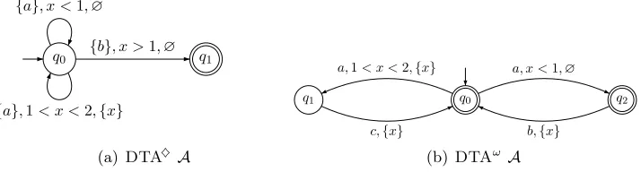
q0 q1
{a}, x <1,∅
{a},1< x <2,{x} {b}, x >1,∅
(a)DTA♦ A
q0 q2
q1
a, x <1,∅
b,{x}
a,1< x <2,{x}
c,{x}
[image:8.612.117.474.111.207.2](b)DTAω A
Figure 3: DTA with (a) reachability and (b) Muller acceptance conditions
constraints likex−y ⊲⊳ care not considered. This restriction does, however, not harm the expressiveness [9].
An (infinite)timed path of DTA A is of the formθ=q0−−−−→a0,t0 q
1−−−−→ · · ·a1,t1 such that
η0 =~0, and for all j>0, it holdstj >0, ηj+tj |=gj,ηj+1 = (ηj+tj)[Xj := 0], where ηj is
the clock evaluation when entering qj. The definitions on timed paths (such as θ[i], θ@t,
and so forth) for CTMCs can readily be adapted for DTA. We consider DTA with two types of acceptance criteria. LetDTA♦ and DTAω denote the set of DTAwith reachability and
Muller acceptance conditions, respectively. DTA denotes the general case covering both DTA♦ and DTAω.
Definition 2.5 (DTA accepting paths). An infinite timed path θ is accepted by a DTA♦
if θ[i]∈QF for some i>0; θ is accepted by a DTAω if inf(θ) ∈QF, where inf(θ) is the
set of states q∈Qsuch thatq =qi for infinitely manyi>0.
The timed path θ is accepted according to a reachability criterion if it reaches some final location, whereas it is accepted according to a Muller acceptance condition if the set of infinitely visited locations equals some set inQF. As a convention, we assume each location
q∈QF inDTA♦ to be a sink.
Example 2.6. Figure 3(a) depicts an example DTA♦ over the alphabet {a, b} with initial
locationq0. The timed automaton is deterministic asq0is the only initial location and both
a-labeled edges have disjoint guards. Any timed path ending inQF ={q1} is accepting.
Figure 3(b) depicts an exampleDTAω over the alphabet{a, b, c}. Its initial location is
q0; its Muller acceptance family equals QF ={q0, q2} . Any accepting path should cycle
between the locations q0 and q1 finitely often, and between q0 and q2 infinitely often.
Remark 2.7. [Expressive power ofDTAω]DTAω is the set of (deterministic) timed Muller
automata, (D)MTA, for short. A (deterministic) timed B¨uchi automaton, (D)TBA for short, has a set QF of accepting locations, and accepts an infinite timed path θ if θ visits
some location inQF infinitely often, i.e., inf(θ)∩QF 6=∅. The expressive power of(D)TMA
and (D)TBAis related as follows [1]:
TMA=TBA>DTMA>DTBA.
Note that in nondeterministic TMA and TBA, guards on edges emanating from a loca-tion may overlap. DTMAare closed under all Boolean operators (union, intersection, and complement), whileDTBAare not closed under complement.
2.3. Piecewise-deterministic Markov processes. PDPs [15] constitute a general model for stochastic systems without diffusions [16] and has been applied to a variety of problems in engineering, operations research, management science, and economics. Powerful analysis and control techniques for PDPs have been developed [23, 24, 13]. A PDP is a hybrid
stochastic process involving discrete control (i.e., locations) and continuous variables. Let us introduce some auxiliary notions. Let X = {x1, . . . , xn} be a set of variables
in R. Note that clock variables are a special case of these variables. A constraint over
X, denoted by g, is a subset of Rn. Let B(X) denote the set of constraints over X. An
X-valuationη satisfies constraintg, denotedη|=g, if and only if (η(x1), ..., η(xn))∈g. For
g ∈ B(X), a constraint over X ={x1, . . . , xn}, let g be the closure of g, ˚g the interior of
g, and ∂g = g\˚g the boundary of g. For instance, for g = x21−2x2 61.5∧x3>2, we
have ˚g =x21−2x2 <1.5∧x3 >2, g=x12−2x2 61.5∧x3 >2, and ∂g equals x21−2x2 =
1.5∧x3 = 2.
To each control location z of a PDP, an invariant Inv(z) is associated, a constraint over X which constrains the variable values in z. The state of a PDP is a pair (z, η) with control location z and η a variable valuation. Let S ={(z, η)|z∈Z, η|=Inv(z)}, where Z is the set of locations. The notions of closure, interior and boundary can be lifted to S in a straightforward manner, e.g., ∂S=Sz∈Z{z} ×∂Inv(z) is the boundary of S; ˚S and S are defined in a similar way.
Definition 2.9 (PDP[16]). A piecewise-deterministic (Markov) process (PDP) is a tuple Z = (Z,X,Inv, φ,Λ, µ) where Z is a finite set of locations, X is a finite set of variables,
Inv :Z→ B(X) is aninvariant function, and
• φ:Z× V(X)×R→ V(X) is aflow function, which is the solution of a system of ODEs with a Lipschitz continuous vector field,
• Λ :S→R>0 is anexit rate function satisfying for any ξ∈S:
∃ǫ(ξ)>0.functiont7→Λ(ξ⊕t) is integrable on [0, ǫ(ξ)), (△) where (z, η)⊕t= z, φ(z, η, t), and
• µ: ¯S→Distr(S) is the transition probability function satisfying:
µ(ξ,{ξ}) = 0 and ξ 7→µ(ξ, A) is measurable for anyA∈ F(S),
where µ(ξ, A) denotes (µ(ξ))(A), F(S) is a σ-algebra generated by Sz∈Z{z} ×Az with
Az ⊆ F(Inv(z)), and F(Inv(z)) is aσ-algebra generated byInv(z).
Let us explain the behavior of a PDP. A PDP can reside in a state ξ = (z, η) ∈˚S as long as Inv(z) holds. In state ξ = (z, η), the PDP can either delay or take a Markovian jump.
Delaying by ttime units yields the next state ξ′=ξ⊕t, i.e., the PDP remains in location z while all its continuous variables are updated according toφ(z, η, t). The flow functionφ defines the time-dependent behavior in a single location, in particular, it specifies how the variable valuations change when time elapses. In case of a Markovian jump in state ξ, the next state ξ′′= (z′′, η′′)∈Sis reached with probability µ(ξ,{ξ′′}). The residence time of a state is exponentially distributed; this is defined by the function Λ. A third possibility for a PDP to evolve is by takingforced transitions. When the variable valuation ηsatisfies the boundary of the invariant, i.e., η |=∂Inv(z), the PDPis forced to take a boundary jump,
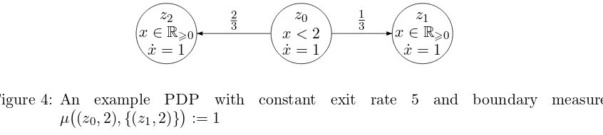
z0
x <2 ˙
x= 1
1
3 z1
x∈R>0 ˙
x= 1
z2
x∈R>0 ˙
x= 1
[image:10.612.96.519.116.211.2]2 3
Figure 4: An example PDP with constant exit rate 5 and boundary measure
µ (z0,2),{(z1,2)} := 1
A PDP is named piecewise-deterministic because in each location (one piece) the
be-havior is deterministically determined by the flow function φ. The PDP is Markovian as the current state contains all the information to determine the future progress of the PDP.
2.4. Embedded PDP. The embeddeddiscrete-time Markov process (DTMP)emb(Z) of thePDPZ has the same state space SasZ and is equipped with a transition probability function ˆµ. The one-jump transition probability from a state ξ to a set A ⊆ S of states (with different location as ξ), denoted ˆµ(ξ, A), is given by [16]:
ˆ
µ(ξ, A) =
Z ♭(ξ)
0
(Q1A)(ξ⊕t)·Λ (ξ⊕t)e−
Rt
0Λ(ξ⊕τ)dτ dt (2.2)
+ (Q1A)(ξ⊕♭(ξ))·e−
R♭(ξ)
0 Λ(ξ⊕τ)dτ (2.3)
where ♭(ξ) = inf{t >0|ξ⊕t∈∂S} is the minimal time to hit the boundary if such time exists; ♭(ξ) = ∞ otherwise. (Q1A)(ξ) =RS1A(ξ′)µ(ξ, dξ′) is the accumulative (one-jump)
transition probability fromξ toAand1A(ξ) is the characteristic function such that1A(ξ) =
1 when ξ ∈ A and 1A(ξ) = 0 otherwise. Term (2.2) specifies the probability to delay to
state ξ⊕t (on the same location) and take a Markovian jump from ξ⊕t to A. Note the delay t can take a value from [0, ♭(ξ)). Term (2.3) is the probability to stay in the same location for♭(ξ) time units and then it is forced to take a boundary jump from ξ⊕♭(ξ) to A sinceInv(z) will be by any delay invalid.
Example 2.10. Figure 4 depicts a 3-locationPDP Z withX =x, whereInv(z0) =x <2
and Inv(z1) = Inv(z2) = x ∈ R>0. Solving ˙x = 1 yields the flow function φ(zi, η(x), t) =
η(x)+t for i = 0,1,2. The state space of Z is S = {(z0, η) | η(x) < 2} ∪ {(z1,R>0)} ∪
{(z2,R>0)}. Let exit rate Λ(ξ) = 5 for anyξ∈S. Forη |=Inv(z0), letµ (z0, η),{(z1, η)} := 1
3,µ (z0, η),{(z2, η)}
:= 23 and the boundary measure be given asµ (z0,2),{(z1,2)}:= 1.
The time for ξ0 = (z0,0) to hit the boundary is ♭(ξ0) = 2. For set of states A={(z1,R)}
and state ξ0, (Q1A)(ξ0⊕t) = 13 if t<2, and (Q1A)(ξ0 ⊕t) = 1 if t=2. This yields for the
transition probability from stateξ0 to A inemb(Z) is:
ˆ
µ(ξ0, A) =
Z 2
0
1 3·5·e
−R0t5 dτ dt+ 1·e−R025 dτ = 1
3 + 2 3e
−10.
3. The Product of a CTMC and a DTA
In this section, we will make the first steps towards the quantitative and qualitative verification of CTMCs against linear real-time properties specified by DTA. The aim is
Pr(C |= A). We first prove that this question is well-defined, i.e., that this set of paths is measurable. The next step is to define the product of a CTMC C and a DTA A. As we will see, this is neither a CTMC nor a DTA, but a mixture of the two. We define the semantics of such products and define a probability space on their paths. The central result of this section is that Pr(C |=A) equals the reachability probability in the product ofC and
A, cf. Theorem 3.10. In order to facilitate the effective computation of these reachability probabilities, we adapt the region construction of timed automata to the product C ⊗ A, and show that this yields a PDP. The analysis of these PDPs will be the subject of the next two sections.
To simplify the notations, we assume w.l.o.g. that a CTMC has a single initial state
s0, i.e., α(s0) = 1, and α(s) = 0 for s 6= s0. The state labels of the CTMC will act as
input symbols of the DTA. Thus, the alphabet of DTA equals the powerset of the atomic propositions, i.e., 2AP
. A timed path in a CTMC is accepted by a DTAA if there exists a corresponding accepting path inA.
Definition 3.1 (CTMC paths accepted by a DTA). LetCTMC C = (S,AP, L, s0,P, E)
and DTAA= (2AP,X, Q, q0, QF,→). TheCTMCpaths0−−→t0 s
1−−→t1 s2· · · isaccepted by A if there exists a correspondingDTApath
q0−−−−−−→L(s0),t0 succ qg 0, L(s0), g0
| {z }
=q1
L(s1),t1
−−−−−−→ succ qg 1, L(s1), g1
| {z }
=q2
· · ·
which is accepted by A, where η0 =~0, gi is the (unique) guard in qi such that ηi+ti |=gi
and ηi+1 = (ηi+ti)[Xi:= 0], and ηi is the clock evaluation when entering qi, for all i.
3.1. Measurability. The quantitative verification of CTMCC against DTA A amounts
to compute the probability of the set of paths in C that is accepted by A. Formally, let
PathsC(A) = {ρ∈PathsC |ρ is accepted byDTA A }.
We first prove its measurability:
Theorem 3.2. For any CTMC C and DTA A, PathsC(A) is measurable.
Proof. It suffices to show that PathsC(A) can be written as a finite union or intersection of measurable sets. The proof is split in two parts: DTA with (1) reachability acceptance, and (2) Muller acceptance. The proof of the first case is carried out by (1a) considering DTA that only contain strict inequalities as guards, (1b) equalities, and (1c) non-strict inequalities. (Note that constraint x=K can be obtained by x > K∧x≥K).
(1a): Let DTA♦ A only contain strict inequalities as clock constraints. As all accepting
paths are finite, PathsC(A) = Sn∈NPathsCn(A), where PathsCn(A) is the set of paths of length n accepted by A. Let ρ = s0−−→t0 s1· · ·sn−1−−−−→tn−1 sn ∈ PathsCn(A). Then
there exists a corresponding path θ=q0−−−−−−→L(s0),t0 q1· · ·qn−1−−−−−−−−−→L(sn−1),tn−1 qn of A which
is induced by the sequence:
q0−−−−−−−−→L(s0),g0,X0 q1· · ·qn−1−−−−−−−−−−−−−→L(sn−1),gn−1,Xn−1 qn,
with qn ∈ QF such that there exist {ηi}06i<n with 1) η0 =~0; 2) ηi+ti |= gi; and 3)
We prove the measurability of PathsCn(A) by showing that for any path ρ =s0−−→ · · ·t0 −−−−→tn−1 sn∈PathsCn(A),
there exists a cylinder set C(s0, I0, . . ., In−1, sn) (Cρ for short) such that:
ρ ∈Cρ and Cρ⊆PathsnC(A) for |ρ|=n. (3.1)
This is proven in two steps:
a. (ρ ∈ Cρ.) Let ρ = s0−−→ · · ·t0 −−−−→tn−1 sn ∈ PathsCn(A). We define Cρ by considering
intervals Ii with rational bounds that are based on ti. Let Ii = [t−i , t+i ] such that
t−i =t+i :=ti if ti ∈Q, and t−i , t+i ∈Qotherwise, such that:
t−i 6ti 6t+i , ⌊t−i ⌋=⌊ti⌋, ⌈t+i ⌉=⌈ti⌉, and t+i −t−i <
∆ 2·n
where ∆ = min
06j<n, x∈X
n
{ηj(x)+tj},1 − {ηj(x)+tj}
{ηj(x)+tj} 6= 0
o
, with {·}
denoting the fractional part. Since DTAA only contains strict inequalities, for anyi withηi+ti|=gi, it follows {ηi(x)+ti} 6= 0.
b. (Cρ ⊆ PathsCn(A).) Let ρ′ := s0 t
′ 0
−−→ · · · t
′
n−1
−−−−→sn ∈ Cρ. Let η0′ := ~0 and η′i+1 :=
(ηi′+t′i)[Xi := 0]. It remains to show that η′i+t′i |=gi. Observe that η′0 =η0, and for
any i >0 and clock variablex,
η′i(x)−ηi(x) 6 i−1
X
j=0
t′j−tj 6 i−1
X
j=0
t+j −t−j 6 n·(t+j −t−j ) 6 ∆
2.
Given that guard gi only contains strict inequalities, it follows η′i+t′i |=gi. This can
be seen as follows. Let gi = x > K for some natural K. As |ηi′(x)−ηi(x)| 6 ∆2
and |t′i−ti|< ∆2, it follows |(ηi′(x)+t′i)−(ηi(x)+ti)|< ∆. Note thatηi(x)+ti > K,
and thus ηi(x)+ti− {ηi(x)+ti} = ⌈ηi(x)+ti⌉ ≥K. Hence, ηi(x)+ti−∆≥ K since,
by definition, ∆ 6{ηi(x) +ti}. It follows that ηi′(x) +t′i > K. A similar argument
applies to the case x < K and extends to conjunctions of strict inequalities. Thus, η′
i+t′i|=gi, and ρ′∈PathsCn(A).
By (3.1) and the fact that PathsCn(A)⊆Sρ∈PathsC
n(A)Cρ, we have: PathsCn(A) = [
ρ∈PathsC
n(A)
Cρ and PathsC(A) =
[
n∈N
[
ρ∈PathsC
n(A)
Cρ.
As each interval in Cρ has rational bounds,Cρ is measurable. It follows that PathsC(A)
is a union of countably many cylinder sets, and hence is measurable.
(1b): Consider DTA♦ A with equalities of the form x =K for natural K. Measurability
is shown by induction on the number of equalities in A. The base case (only strict inequalities) has been shown above. Now suppose there exists an edge e=q−−−−→a,g,X q′ in Awheregcontains the constraintx=K. LetDTA♦ Aebe obtained fromAby deleting
all the outgoing edges from q except e. We then consider the DTA A¯e, A>e, and A<e
where ¯Ae is obtained fromAe by replacingx=K by true;A>e is obtained fromAe by
replacing x=K by x > K and Ae< is obtained from Ae by replacingx=K by x < K.
Since A is deterministic, it follows that
PathsC(Ae) =PathsC( ¯Ae)\ PathsC(A>e)∪PathsC(A<e)
By the induction hypothesis, the sets PathsC( ¯Ae), PathsC(A>e) and PathsC(A<e) are
measurable. Hence, PathsC(Ae) is measurable. Furthermore, as
PathsC(A) = [
e=q−−−−→a,g,X q′
PathsC(Ae),
where all guardsg of edge eare equalities, it follows that PathsC(A) is measurable. (1c): Let DTA♦ A have clock constraints of the form x ⊲⊳ K where ⊲⊳∈ {≥,≤}. We
consider theDTAA=andA⊲⊳, whereA= is obtained fromAby changing all constraints
of the form x ⊲⊳ K by x =K, and A⊲⊳ is obtained from A by changing any constraint
x ⊲⊳ K byx ⊲⊳ K, with≥=>and≤=<otherwise. Clearly,PathsC(A) =PathsC(A=)∪
PathsC(A⊲⊳). As it was shown before thatPathsC(A=) andPathsC(A⊲⊳) are measurable,
it follows that PathsC(A) is measurable.
(2): Let DTAωA with QF = {F1, . . . , Fk}. PathsC(A) = T
0<i6kPathsi where Pathsi is
the set of paths in CTMC C whose corresponding DTA paths are accepted by Fi ∈QF,
i.e., Pathsi={θ∈PathsC(A)|inf(θ) =Fi}. We have:
Pathsi= \
n>0
[
m>n
[
s0,...,sn,sn+1...,sm
C(s0, I0, . . . , In−1, sn, . . . , Im−1, sm),
where{sn+1, . . . , sm}=LFi withLFi the set of CTMC states whose corresponding DTA
states are Fi, and C(s0, I0, . . . , In−1, sn, . . . , Im−1, sm) is the cylinder set such that each
timed path of the cylinder set of the form s0−−→ · · ·t0 −−−−→tn−1 sn· · ·−−−−→tm−1 sm is a prefix
of an accepting path of A. It follows that Pathsi is measurable. Thus, PathsC(A) is measurable.
3.2. The product of a CTMC and a DTA. A central step in the verification of a CTMC
C against a DTAA is to construct its synchronous productC ⊗ A. The resulting object is neither a CTMC nor a DTA, but a mixture of the two. We first define this model, called deterministic Markovian timed automata, and define a measurable space over its paths. In Section 4, we consider the computation of Pr(C |=A) = Pr PathsC(A) which is based on this product.
Definition 3.3(DMTA). Adeterministic Markovian timed automaton (DMTA) is a tuple M = (Loc,X, ℓ0, LocF, E, ), where Loc is a nonempty finite set of locations; X is a finite set of clocks; ℓ0 ∈Loc is the initial location; LocF is the acceptance condition with LocF = LocF ⊆ Loc the reachability condition and LocF = LocF ⊆ 2Loc the Muller
condition;E:Loc→R>0 is theexit rate function; and ⊆Loc× CC(X)×2X×Distr(Loc)
is anedge relation such that:
ℓ g,X/o /o /o //ζ and ℓ
g′,X′
/
/
/o
/o
/o ζ′ withg6=g′
implies g∩g′ =∅.
DMTA closely resemble DTA, but have in addition to DTA an exit rate function that determines the random residence time in a location, and an edge relation where the target of an edge is a probability distribution over the locations. Concepts such as clock valuation, clock constraints and so forth are defined as forDTA. We refer to ℓ g,X/o /o /o //ζ for distribution
ζ ∈ Distr(Loc) as an edge and to ℓ g,X
The intuition is that when entering location ℓ, the DMTA chooses a residence time which
is governed by an exponential distribution with rate E(ℓ). Thus, the probability to leaveℓ within ttime units is 1−e−E(ℓ)t. Due to the determinism of the edge relation, at most one
edge, say ℓ g,X/o /o /o //ζ , is enabled. The probability to jump to ℓ′ via this edge equals ζ(ℓ′).
Similar as forDTAs,DMTA♦ and DMTAω are defined andDMTA refers to both classes.
Definition 3.4 (DMTA paths). An (infinite)symbolic path of DMTA M is of the form:
ℓ0
g0,X0
p0
/
/ ℓ
1
g1,X1
p1
/
/ ℓ
2· · · where ℓi
gi,Xi
/
/
/o
/o
/o ζ
i and pi =ζi(ℓi+1), for all i∈N.
A symbolic path induces infinite paths of the form τ = ℓ0−−→t0 ℓ1−−→t1 ℓ2· · · such that
η0 =~0, (ηi+ti)|=gi, andηi+1= (ηi+ti)[Xi := 0] wherei>0 andηi is the clock valuation
of X in Mwhen entering location ℓi. The path τ is accepted by a DMTA♦ if there exists
n>0, such thatτ[n]∈LocF. It is accepted by DMTAω if and only if inf(τ)∈LocF.
DMTA semantics. Consider clock valuation η in location ℓ. As the DMTA is deter-ministic, at most one guard is enabled in state (ℓ, η). The one-jump probability of taking the transition ℓ g,X
p //ℓ′ within time intervalI starting at clock valuation η in location ℓ,
denoted pη(ℓ, ℓ′, I), is defined as follows:
pη(ℓ, ℓ′, I) =
Z
I
E(ℓ)·e−E(ℓ)τ
| {z }
(i) density to leaveℓatτ
· 1g(η+τ)
| {z }
(ii)η+τ|=g?
· p
|{z}
(iii) probabilistic jump
dτ (3.2)
Note the resemblance with (2.1). Actually, part (i) characterizes the delay τ at location ℓ which is exponentially distributed with rate E(ℓ); (ii) is the characteristic function, where 1g(η+τ) = 1 if and only if η+τ |=g. It compares the current valuation η+τ with guard g
and rules out those violating g. Part (iii) indicates the probability of the transition under consideration. Note that (i) and (iii) are features fromCTMCs while (ii) stems fromDTA.
The characteristic function 1g is Riemann integrable as it is bounded and its support is
an interval; therefore,pη(ℓ, ℓ′, I) is well-defined. The one-jump probability can be uniquely
defined in this way because it relates to a fixed clock evaluation η.
The above characterisation of the one-jump probability provides the basis for defining the probability of a set of DMTA paths. Let C(ℓ0, I0, . . ., In−1, ℓn) be the cylinder set with
(ℓ0, . . ., ℓn) ∈ Locn+1 and Ii ⊆ R>0. It denotes a set of paths in DMTA M such that
for any such path τ, τ[i] = ℓi and τhii ∈ Ii. Let PrMη0 (C(ℓ0, I0, . . ., In−1, ℓn)) denote the probability ofC(ℓ0, I0, . . ., In−1, ℓn) such thatη0 is the initial clock valuation in locationℓ0.
Let PrMη0 (C(ℓ0, I0, . . ., In−1, ℓn)) =PM0 (η0), wherePMi (η) is inductively defined as follows:
PMi (η) =
1 if i=n
Z
Ii
E(ℓi)·e−E(ℓi)τ·1gi(η+τ)·pi
| {z }
(⋆)
·PMi+1(η′)
| {z }
(⋆⋆)
dτ if 06i < n, (3.3)
where η′ := (η+τ)[X
i := 0]. Intuitively, PMi (ηi) is the probability of the suffix cylinder
set starting fromℓi and ηi to ℓn. It is recursively defined by the product of the probability
probability of the suffix cylinder set from ℓi+1 and ηi+1 on (cf. (⋆⋆)). For the same reason
aspη(ℓ, ℓ′, I) is well-defined,PMi (η) is well-defined.
Example 3.5. TheDMTA♦ in Figure 5(a) has initial locationℓ
0 with two outgoing edges,
with guards x <1 and 1 < x < 2. We use the small black dots to indicate distributions. Assume t time units elapse inℓ0. If the current clock evaluation η satisfies η(x) <1, then
the upper edge is enabled and the probability to go toℓ1 within timetis p~0(ℓ0, ℓ1,[0, t]) =
(1−e−r0t)·1, whereE(ℓ
0) = r0; no clock is reset. It is similar when 1< η(x) <2, except
thatxwill be reset (cf. the lower edge emanating from locationℓ0). Ifη(x)>2, no outgoing
edge is enabled, and the DMTA stays inℓ0 ad infinitum.
ℓ0=hs0, q0i ℓ1=hs1, q0i
x<1,∅
1 ℓ
2=hs2, q0i
1<x<2,{x}
x<1,∅
0.2
r0 r1
r2
ℓ4=hs3, q0i r3
ℓ3=hs2, q1i
r2
1<x<2,{x}
x>1,∅ 1 0.3
0.5
(a)DMTA♦C ⊗ A
s0 s1
1
0.5
s2
s3
0.2
0.3
1
1
{a} {a}
{b}
{c} r3
r2
r1
r0
(b)CTMCC
q0 q1
{a}, x <1,∅
{a},1< x <2,{x} {b}, x >1,∅
(c) DTA♦A
ℓ0,06x<1 ℓ0,16x<2
ℓ1,06x<1 ℓ1,16x<2
1
1
v0, r0 v1, r0
v2, r1 v3, r1
0.5 δ
reset, 0.5
ℓ2,06x<1 ℓ2,16x<2
ℓ3,16x<2
ℓ2, x>2
ℓ3, x>2
1
v4,0 v5, r2
v7,0
δ
δ
1
v8,0
reset,0.2 0.2
δ
v6, r2
δ
[image:15.612.93.513.282.612.2](d) Reachable region graph ofC ⊗ A
Figure 5: Example productDMTA♦ of CTMC C and DTA♦ A
3.3. Product DMTA. The productC ⊗ AforCTMCC and DTA A, is aDMTA.
Definition 3.6 (Product of CTMCandDTA). LetC= (S,AP, L, s0,P, E) be aCTMC
and A = (2AP
,X, Q, q0, QF,→) be a DTA. Let C ⊗ A = (Loc,X, ℓ0, LocF, E, ) be the
• LocF=LocF :=S×QF, if QF =QF (reachability condition)
• LocF=LocF :=SF∈QFS×F, if QF=QF (Muller condition)
and is defined as the smallest relation defined by the rule: P(s, s′)>0 ∧ q−−−−−−→L(s),g,X q′
hs, qi g,X/o /o /o //ζ
such thatζ(hs′, q′i) =P(s, s′).
The DMTA C ⊗ Ais basically the synchronous product of CTMC C and DTA Asuch that transition s→ s′ in C is matched with the edge q−−−−−−→L(s),g,X q′, i.e., the set of atomic
propositions ofsacts as input symbol for the edge from locationqtoq′inA. The probability of the joint evolvement ofC andA is given byP(s, s′), the discrete probability ofs→s′ in
C, whereas the residence time in the locationhs, qi is given byE(s), the exit rate ofsinC. It is easy to see from the construction that C ⊗ Ais indeed aDMTA. The determinism of
theDTAAguarantees that the induced product is also deterministic. In C ⊗ A, from each
location there is at most one “input symbol” possible, viz.L(s). For the sake of convenience, input symbols can be omitted from C ⊗ A.
Example 3.7. LetCTMC Cand DTA♦ A be given in Figure 5(b) and 5(c), respectively.
The product DMTA♦ C⊗A is depicted in Figure 5(a). SinceQ
F ={q1} inA, the set of
accepting locations in DMTA♦ is LocF ={hs2, q1i}={ℓ3}.
Example 3.8. For the CTMC C in Figure 6(a) and the DTAω A in Figure 6(b) with
acceptance family QF = {q1, q2},{q3, q4} , the product DMTAω C ⊗ A is shown in
Figure 6(c). LocF = {hsi, q1i,hsj, q2i},{hs′i, q3i,hs′j, q4i} , for any si, s′i, sj, s′j ∈ S, i.e.,
LocF ={ℓ1, ℓ2, ℓ3},{ℓ4, ℓ5, ℓ6} .
The set of accepted paths in DMTAC⊗A is defined by:
AccPathsC⊗A := {τ ∈PathsC⊗A |τ is accepted by C⊗A }.
For n-ary tuple J, let J⇂i denote the i-th entry in J, for 1 6 i 6 n. For a (C⊗A
)-path τ = hs0, q0i−−→ ht0 s1, q1i−−→ · · ·t1 , let τ⇂1 := s0−−→t0 s1−−→ · · ·t1 , and for any set Π of
(C⊗A)-paths, let Π⇂1 =Sτ∈Πτ⇂1. The following lemma asserts that there is a one-to-one
relationship between paths in CTMCC accepted by DTAAand accepting paths in C ⊗ A. Lemma 3.9. For any CTMC C and DTA A, PathsC(A) = AccPathsC⊗A⇂1.
Proof. We provide the proof forDTA♦ A; the proof for DTAω A is similar.
(⊆) Letρ∈PathsC(A). We prove that there exists a pathτ ∈AccPathsC⊗A withρ=τ⇂1.
Assume w.l.o.g. that ρ = s0−−→t0 s1· · ·sn−1−−−−→tn−1 sn ∈ PathsC(A), i.e., sn ∈ QF, η0 |=~0,
and for 06i < n,ηi+ti |=gi and ηi+1 = (ηi+ti)[Xi := 0], where ηi is the clock valuation
inA when entering statesi in C. We construct a timed path θ∈PathsA from ρ such that
θ=q0−−−−−−→L(s0),t0 q1· · ·qn−1−−−−−−−−−→L(sn−1),tn−1 qn, where the clock valuation on enteringsi and qi
coincides. From ρand θ, we can now construct the path
τ =hs0, q0i−−→ ht0 s1, q1i · · · hsn−1, qn−1i−−−−→ htn−1 sn, qni,
s1
s2
s0
1
0.3 0.4
s3
0.6
0.7
1
r0,{b}
r3,{c}
r2,{a}
r1,{c}
(a) CTMCC
q0 q3 q4
q1
q2 b,1<x<2,∅
b, x<1,{x}
c, x <2,{x}
a, x >1,∅
c, x >1,∅
a, x >2,{x}
(b)DTAω Aω
ℓ0=hs0, q0i
ℓ1=hs1, q3i
ℓ2=hs3, q3i
ℓ3=hs2, q4i
ℓ4=hs1, q1i
ℓ5=hs3, q1i
ℓ6=hs2, q2i
x<1,{x} 1<x<2,∅
0.4
0.6
0.4
0.6 0.3
0.7
x >1,∅
0.3
0.7
x >2,{x}
r0
r1
r3
r2
r1
r3
r2
x >1,∅
1
x >1,∅
1
x <2,{x}
1
x <2,{x}
1
[image:17.612.113.492.125.378.2](c)DMTAω C ⊗ Aω
Figure 6: Example productDMTAω of CTMCC and DTAω Aω
(⊇) Letτ ∈AccPathsC⊗A. We prove that τ⇂1∈PathsC(A). Assume w.l.o.g. that
τ =hs0, q0i−−→ · · ·t0 −−−−→ htn−1 sn, qni ∈AccPathsC⊗A,
with hsn, qni ∈LocF, η0 |=~0, and for 0 6 i < n, ηi+ti |=gi and ηi+1 = (ηi+ti)[Xi := 0],
whereηi is the clock valuation when entering location hsi, qii. It then directly follows that
qn∈QF andτ⇂1 ∈PathsC(A), given the entering clock valuation ηi of state si.
Theorem 3.10. For any CTMC C and DTA A,
PrC PathsC(A) = Pr~C⊗A
0 AccPaths C⊗A.
Proof. We provide the proof forDTA♦ A; the proof for DTAω A goes along similar lines
as in the proof of Theorem 3.2.
According to Theorem 3.2, PathsC(A) can be rewritten as the combination of cylinder sets of the form C(s0, I0, . . . , In−1, sn) which are all accepted by DTA♦ A. Note that this
means that each path in the cylinder set is accepted byA. By Lemma 3.9, namely by path lifting, we can establish exactly the same combination of cylinder setsC(ℓ0, I0, . . . , In−1, ℓn)
for AccPathsC⊗A, where si = ℓi⇂1. It then suffices to show that for each cylinder set
C(s0, I0, . . . , In−1, sn) which is accepted byA, PrC and PrC⊗A yield the same probabilities.
For the measure PrC, according to Eq. (2.1) (cf. page 5),
PrC C(s0, I0, . . . , In−1, sn)=
Y
06i<n
Z
Ii
The measure Pr~C⊗A
0 , according to Section 3.2, is given byP C⊗A
0 (~0), wherePC⊗An (η) = 1
for any clock valuation η and for any 06i < n:
PC⊗Ai (ηi) =
Z
Ii
1gi(ηi+τi)·pi·E(ℓi)·e
−E(ℓi)τi ·PC⊗A
i+1 (ηi+1) dτi,
whereηi+1= (ηi+τi)[Xi := 0] and1gi(ηi+τi) = 1, ifηi+τi|=gi; 0, otherwise.
We will show, by induction, thatPC⊗Ai (ηi) is a constant, i.e., is independent ofηi, if the
cylinder setC(ℓ0, I0, . . . , In−1, ℓn) is accepted byC ⊗ A. First note that for this cylinder set
there must exist some sequence of transitions
ℓ0 g0,X0
p0
/
/ ℓ
1 · · · ℓn−1
gn−1,Xn−1
pn−1
/
/ ℓ
n
with η0 =~0 and ∀ti ∈ Ii with 0 6 i < n, ηi+ti |= gi and ηi+1 := (ηi +ti)[Xi := 0].
Moreover, according to Definition 3.6, we have:
pi=P(si, si+1) and E(ℓi) =E(si). (3.4)
We apply a backward induction onndown to 0. The base case is trivial sincePC⊗An (ηn) = 1.
By the induction hypothesis, PC⊗Ai+1 (ηi+1) is a constant. For the induction step, consider
i < n. For any τi∈Ii, sinceηi+τi |=gi,1gi(ηi+τi) = 1, it follows that
PC⊗Ai (ηi) =
Z
Ii
1gi(ηi+τi)·pi·E(ℓi)·e
−E(ℓi)τi·PC⊗A
i+1 (ηi+1) dτi
I.H.
=
Z
Ii
pi·E(ℓi)·e−E(ℓi)τidτi·PC⊗Ai+1 (ηi+1)
Eq.(3.4)
=
Z
Ii
P(si, si+1)·E(si)·e−E(si)τidτi·PC⊗Ai+1 (ηi+1).
Clearly, this is a constant. It is thus easy to see that
Pr~C⊗A
0 C(ℓ0, I0, . . . , In−1, ℓn)
:= PC⊗A0 (~0) = Y
06i<n
Z
Ii
P(si, si+1)·E(si)·e−E(si)τdτ,
which completes the proof.
3.4. Region graph construction. Theorem 3.10 asserts that the probability of CTMC
C satisfying the DTA specification A equals the reachability probability of some accepting location in C ⊗ A. The state space of C ⊗ A, however, is infinite. As a next step towards obtaining an effective procedure for computing reachability probabilities inC ⊗ Awe adopt the standard region construction of timed automata [1] to DMTA. This yields a stochastic
process, namely a PDP. Here, we consider the region construction for finite acceptance conditions, i.e,DMTA♦. The details forDMTAω are slightly different (only the acceptance
set differs) and are provided in Section 5.
Let us briefly recall the concept of a region. Formally, a region is an equivalence under
∼
=, an equivalence relation on clock valuations. A region is characterized by a specific form of a clock constraint. Let cxi be the largest constant with which xi ∈ X is compared in
some guard in the (DM)TA. Clock evaluations η, η′ ∈ V(X) are clock-equivalent, denoted η∼=η′, if and only if either
(2) for any xi, xj ∈ X withη(xi), η′(xi)6cxi and η(xj), η′(xj)6cxj it holds:
⌊η(xi)⌋=⌊η′(xi)⌋ and {η(xi)}6{η′(xi)}iff η(xj)6η′(xj),
where⌊d⌋and {d}are the integral and fractional part of d∈R, respectively. This clock equivalence is coarser than the traditional definition by merging the “bound-ary” regions (those with point constraints like “x = 0”) into the “non-boundary” regions (those only with interval constraints like “0< y < 1”). For instance, forX ={x1, x2}, the
boundary regions (x1 = 0, x2 = 0), (0< x1 <1, x2 = 0) and (x1= 0,0< x2 <1) are merged
with the non-boundary region (0< x1 <1,0< x2 <1) yielding (06x1 <1,0 6x2 <1).
The reason for this slight change will become clear later.
Let Re(X) be the set of regions over the set X of clocks. For Θ,Θ′ ∈ Re(X), Θ′ is the successor region of Θ if for all η |= Θ there exists δ ∈ R>0 such that η+δ |= Θ′ and
∀δ′ < δ. η+δ′ |= Θ∨Θ′. The region Θ satisfies the guard g, denoted Θ |=g, iff ∀η |= Θ.
η|=g. Thereset operation on region Θ is defined as Θ[X:= 0] :=η[X := 0]|η|= Θ .
Definition 3.11(Region graph ofDMTA♦). Theregion graphof DMTA♦M= (Loc,X, ℓ 0,
LocF, E, ) is G(M) = (V, v0, VF,Λ, ֒→), where
• V =Loc× Re(X) is a finite set ofvertices withinitial vertex v0 = (ℓ0,~0); • VF =v∈V |v⇂1∈LocF is the set ofaccepting vertices;
• Λ :V →R>0 is the exit rate function where:
Λ(v) =
(
E(v⇂1) if v
p,X
֒→ v′ for somev′ ∈V
0 otherwise.
• ֒→ ⊆ V × [0,1]×2X∪ {δ}×V is the transition (edge) relation, such that:
◮ v֒→δ v′ if v⇂1 =v′⇂1, andv′⇂2 is the successor region ofv⇂2;
◮ vp,X֒→ v′ if v⇂1 g,X
p //v′⇂
1 with v⇂2 |=g, and v⇂2[X:= 0] =v′⇂2.
Any vertex in the region graph is a pair consisting of a location and a region. Edges of the form v ֒→δ v′ are called delay edges, whereas those of the form v p,X֒→ v′ are called Markovian edges. Note that Markovian edges emanating from a boundary region do not
contribute to the reachability probability as the time to hit the boundary is always zero (i.e., ♭(v, η) = 0 in Eq. (4.3), page 20). Therefore, we can safely remove all the Markovian edges emanating from boundary regions and combine each such boundary region with its unique non-boundary (direct) successor. In the sequel, by slight abuse of notation, we refer to thissimplified region graph asG(M). Note that thenv⇂2[X:= 0]⊆v′⇂2 in the last item
of Definition 3.11.
Remark 3.12. [Exit rates] The exit rate Λ(v) equals 0 if only delay transitions emanate
from v. The probability to take the delay edge within time t is e−Λ(v)t = 1, while the
probability to take Markovian edges is 0.
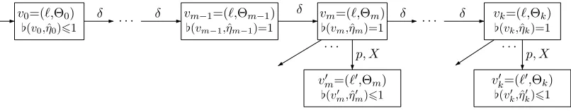
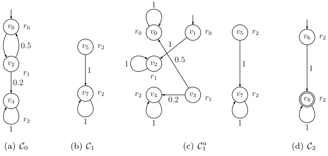
Example 3.13. For theDMTA♦C⊗Ain Figure 5(a), the reachable part (forward reachable
from the initial vertex and backward reachable from the accepting vertices) of the simplified region graphG(C⊗A) is shown in Figure 5(d). Note that the exit rates on v4 and v7 are 0,
The following result asserts that the region graph obtained from a DMTA is in fact a PDP. This is an important observation, as verification now reduces to analyzing this PDP. Lemma 3.14. The region graph of any DMTA induces a PDP.
Proof. LetDMTA♦M= (Loc,X, ℓ0, LocF, E, ) with region graphG(M) = (V, v0, VF,Λ,
֒→). Define Z(M) = (V,X,Inv, φ,Λ, µ) where for any v∈V:
• Inv(v) :=v⇂2 and the state space S:=(v, η)|v∈V, η|=Inv(v) ;
• φ(v, η, t) :=η+t;
• Λ(v, η) := Λ(v);
• if v֒→δ v′ inG(M), then µ((v, η),{(v′, η)}) := 1, provided η|=∂Inv(v);
• if vp,X֒→ v′ inG(M), then µ((v, η),{(v′, η[X := 0])}) :=p, providedη |=Inv(v). It follows directly thatZ(M) is a PDP.
Note that the acceptance conditions play no role in the definition of a PDP, thus this lemma applies to bothDMTA♦ andDMTAω.
4. Verifying CTMCs Against Finite DTA Specifications
The characterization of the region graph of C ⊗ A as a PDP paves the way to the verification of CTMC C against DTA♦ specification A. This section concentrates on the
quantitative verification problem and deals with single-clock DTA separately.
4.1. Quantitative verification with arbitrarily many clocks. The central issue in quantitative verification is to compute the probability of the set of paths in C accepted by A. By Theorem 3.10, this is equal to computing reachability probabilities in DTMA
C ⊗ A. The remaining question is how to determine these probabilities. To that end, we
show that this amounts to determine reachability probabilities of untimed events in the embedded PDP ofZ(C ⊗ A) (cf. Theorem 4.3 below). These probabilities are characterized by a Volterra integral equation system of second type. As solving this integral equation system is typically hard, we present an effective approximation algorithm.
Characterizing reachability probabilities. We first consider determining unbounded reachability probabilities in the PDP Z = Z(C ⊗ A). This is done by considering its
embedded PDP, the DTMPemb(Z), as for unbounded reachability probabilities, the timing aspects are not important. Note that the set of locations of PDPZ andemb(Z) are equal. Besides, the discrete probabilistic evolution ofZandemb(Z) coincide. The main difference is that emb(Z) is time-abstract whereasZ is not.
Let initial state (v0,~0) and T ⊆ V be the set of goal locations. For state (v, η), let
Probemb(Z) (v, η), T, Probv(η, T) for short, denote the probability to reach some state in
(T,·) from state (v, η) inemb(Z). These probabilities are recursively defined as follows. For vertex v∈V, we have:
Probv(η, T) =
(
1 if v∈T
Probv,δ(η, T) +P
vp,X֒→v′Probv,v′(η, T) otherwise
(4.1)
For a delay transitionv֒→δ v′ we have:
Probv,δ(η, T) = e−Λ(v)·♭(v,η)·Probv′ η+♭(v, η), T, (4.2) where e−Λ(v)·♭(v,η) is the probability to stay in v for at most ♭(v, η) time units. Recall
that ♭(v, η) is the minimal time for state (v, η) to hit the boundary ∂Inv(v). Stated in
other words, e−Λ(v)·♭(v,η) is the probability to reside in v without violating the invariant.
The reachability probability from the resulting state η+♭(v, η) is then given by the second multiplicand in Eq. (4.2). This equation is based on Eq. (2.3) by determining the multi-step reachability probability using a sequence of one-step transition probabilities.
For the Markovian transition vp,X֒→ v′, we have:
Probv,v′(η, T) =
Z ♭(v,η)
0
p·Λ(v)·e−Λ(v)·τ·Probv′ (η+τ)[X:= 0], T dτ. (4.3)
Here, Λ(v)·e−Λ(v)·τ denotes the density to stay for exactly τ time units in v. As any delay up to♭(v, η) does not violate the invariant,τ ranges over the dense interval [0, ♭(v, η)]. The state after first delaying τ time units and then taking the edge v p,X֒→ v′ is (η+τ)[X := 0].
Eq. (4.3) is derived from Eq. (2.2).
ℓ0=hs0, q0i ℓ1=hs1, q1i r0 x2>1,{x1} 1 r1
x1<2,{x2} 1
(a)DMTA♦C ⊗ A
v0,0 v1, r0 v2, r0
v3,0
1,{x1}
δ δ
1,{x1}
v4,0
ℓ0 06x1=x2<1
ℓ0 16x1=x2<2
ℓ0
x1>2, x2>2
ℓ1 06x1<1 16x2<2
x2>x1+1
ℓ1 06x1<1
x2>2
x2>x1+2
[image:21.612.161.445.380.579.2](b) Reachable region graphG(C ⊗ A)
Figure 7: Reachable fragment of its region graph
Example 4.1. Consider theDMTA♦in Figure 7(a) and its region graph in Figure 7(b). Let
T =VF be the set of goal locations, i.e., the set of target states{(v, η)|v∈VF, η|=Inv(v)}.
The system of integral equations forv1 in locationℓ0 is as follows. For 16x1 =x2 <2:
Probv1(x1, x2) =Probv1,δ(x1, x2) +Probv1,v3(x1, x2), where
Probv1,δ(x1, x2) =e
−(2−x1)r0·Prob
and
Probv1,v3(x1, x2) =
Z 2−x1
0
r0·e−r0τ·Probv3(0, x2+τ) dτ
whereProbv3(0, x2+τ) = 1. The integral equations for vertices v2, v4 are similar.
Remark 4.2. Clock valuations η and η′ in region Θ may induce different reachability
probabilities. This is due to the fact that η and η′ may have different periods of time to hit the boundary, Thus, the probability for η and η′ to either delay or take a Markovian transition may differ. This is in contrast with timed automata, as well as probabilistic extensions thereof [22], where clock valuations in the same region are not distinguished.
Hence, reachability probabilities in the embedded PDP ofZ(C ⊗A) are characterized by a system of Volterra integral equations (4.1). One can read (4.1) either in the formf(ξ) =
R
Dom(ξ)K(ξ, ξ′)f(dξ′), where K is the kernel and Dom(ξ) is the domain of integration
depending on the continuous state spaceS; or in the operator form f(ξ) = (Jf)(ξ), where
J is the integration operator. Generally, (4.1) does not necessarily have a unique solution. It turns out that the reachability probability Probv0(~0) coincides with the least fixpoint of the operatorJ (denoted by lfpJ) i.e., Probv0(~0) = (lfpJ)(v0,~0).
Theorem 4.3. For any CTMC C and DTA♦ A,
Pr~C⊗A
0 AccPaths
C⊗A is the least solution of ProbD
v0(~0, VF),
where DTMP D=emb(Z(C ⊗ A)).
Proof. Let Pr~C⊗A
0 AccPaths
C⊗A be the least solution of the system of integral equations:
Pr(ℓ, η) =
1 if ℓ∈LocF
Z ∞
0
E(ℓ)·e−E(ℓ)τ · X
ℓ g,X
p
/
/ℓ′
1g(η+τ)·p·Pr(ℓ′,(η+τ)[X := 0])dτ otherwise,
Informally, Pr(ℓ, η) is the probability to reach the set of locationsLocF from locationℓand
clock valuation η. The above integral can be simplifed as follows. W.l.o.g. assume clock constraints to be of the formxEc, where c∈Nand E∈ {≤, <,≥, >}. Then we have:
Pr(ℓ, η) =
Z t2
t1
E(ℓ)·e−E(ℓ)τ · X
ℓ g,X
p
/
/ℓ′
p·Pr(ℓ′,(η+τ)[X := 0])dτ,
wheret1, t2 ∈Q>0∪ {∞} and η+τ |=g for any t1< τ < t2.
If ℓ ∈ LocF, the theorem follows directly. In the remainder of the proof, assume
ℓ /∈LocF. Our proof is based on showing that for anyℓ /∈LocF and clock valuation η,
Pr(ℓ, η) = Probv0(η, VF), (4.4)
where v0 is the initial vertex in the region graph Z(C ⊗ A) with v0⇂1 =ℓ, and VF ={v ∈
to reach LocF in n steps in C ⊗ A. For n = 0, we have Prn(ℓ, η) = 1 if ℓ ∈LocF and 0,
otherwise. For n >0, we define inductively:
Prn(ℓ, η) =
Z t2
t1
E(ℓ)·e−E(ℓ)τ · X
ℓ g,X
p //ℓ′
p·Prn−1(ℓ′, η′) dτ.
Similarly, let Probnv(η, VF) be the probability to reach the set of goal states VF in n > 0
steps:
Probnv(η, VF) =
(
Probnv,δ(η, VF) +Probvs,n(η, VF), if v /∈VF
1, otherwise (4.5)
Probs,nv (η, VF) =
Z ♭(v,η)
0
Λ(v)·e−Λ(v)τ· X
vp,X֒→v′
p·Probnv′−1 (η+τ)[X:=0], VF dτ, (4.6)
Probnv,δ(η, VF) = e−Λ(v)♭(v,η)·Probnv′ η+♭(v, η), VF
. (4.7)
In the sequel, we show that for any n∈N, it holds:
Prn(ℓ, η) =Probnv0(η, VF). (4.8)
The theorem then follows from the fact that lim
n→∞Pr
n(ℓ, η) = Pr(ℓ, η) and, similarly,
lim
n→∞Prob
n
v(η, VF) =Probv(η, VF).
· · · ·
v0=(ℓ,Θ0)
♭(v0,ηˆ0)61
vm−1=(ℓ,Θm−1)
♭(vm−1,ηˆm−1)=1
δ δ vm=(ℓ,Θm)
♭(vm,ηˆm)=1
vk=(ℓ,Θk)
♭(vk,ηˆk)=1
δ δ
δ
v′
m=(ℓ′,Θm)
♭(v′ m,ηˆ′m)61
p, X
v′k=(ℓ′,Θk)
♭(v′ k,ηˆ′k)61
p, X
[image:23.612.95.498.413.492.2]· · · ·
Figure 8: The sub-region graph Z(C ⊗ A) for the transition from ℓto ℓ′.
The proof of Prn(ℓ, η) =Probnv0(η, VF) is by induction onn.
(1) (Base case.) Forn= 0, Pr0(ℓ, η) = 0 =Prob0v0(η, VF) if ℓ /∈LocF, and 1 otherwise.
(2) (Induction step.) Consider n+1. Let edge ℓ g,X ζ inC ⊗ A. Assume the fragment of the region graphZ(C ⊗ A) that corresponds to this edge withζ(ℓ, ℓ′)>0 is as shown in Fig. 8. Location ℓinduces the vertices {vi = (ℓ,Θi)|06i6k}. Intuitively speaking,
the transition from location ℓto ℓ′ is enabled in region Θi form6i6k, whereas only
a delay can take place in all regions Θi withi < m(while staying in location ℓ).
Let ˆηi be the clock valuation when entering vertex vi, i.e., ˆη0 =η and ˆηi = ˆηi−1+
♭(vi−1,ηˆi−1) for 0< i6k. It is assumed that ˆηi 6|=g, where g is the guard of the edge
at hand, for i < mand i > k. Accordingly,
t1 =
mX−1
i=0
♭(vi,ηˆi) and t2=
k
X
i=0
♭(vi,ηˆi)
For convenience, let pn
v(η) := Probnv,δ(η, VF) +Probs,nv (η, VF). Given the fact that
only a delay transition can be taken before time t1, it holds that
pnv0+1(η) = e−t1Λ(v0)·pn+1
vm (ˆηm), where
pnvm+1(ˆηm) = Probnvm+1,δ(ˆηm, VF) +Probs,nvm+1(ˆηm, VF).
We now derive:
e−t1Λ(v0)·Probs,n+1
vm (ˆηm, VF)
= e−t1Λ(v0)·
Z ♭(vm,ηˆm)
0
Λ(vm)·e−Λ(vm)τ·
X
vm p,X
֒→v′
m
p·Probnv′
m (ˆηm+τ)[X:= 0], VF
dτ
=
Z t1+♭(vm,ηˆm)
t1
Λ(vm)·e−Λ(vm)τ·
X
vm p,X
֒→v′
m
p·Probnv′
m (ˆηm+τ−t1)[X:= 0], VF
dτ.
Now consider:
pnv0+1(η) =e−t1Λ(v0)·Probn+1
vm,δ(ˆηm, VF) +e
−t1Λ(v0)·Probs,n+1
vm (ˆηm, VF).
Using the definition ofProbnv+1
m,δ(ˆηm, VF) (see Eq. (4.7)), together with the result derived
above, yields the following sum of integrals:
pnv0+1(η) =
kX−m
i=0
Z t1+Pij=0♭(vm+j,ˆηm+j)
t1+Pij−1=0♭(vm+j,ηˆm+j)
Λ(vm+i)·e−Λ(vm+i)τ
· X
vm+i p,X
֒→v′
m+i
p·Probnv′
m+i (ˆηm+i+τ−t1−
i−1
X
j=0
♭(vm+j,ηˆm+j))[X := 0], VF
| {z }
=Fn(τ)
dτ.
UsingFn(t) we obtain:
pnv0+1(η) =
Z t2
t1
Λ(v0)·e−Λ(v0)τ·Fn(τ)dτ. (4.9)
Notice that
ˆ
ηm+i =η+
mX−1
j=0
♭(vj,ηˆj)
| {z }
=t1 +
i−1
X
j=0
♭(vm+j,ηˆm+j).
Therefore, for anyt∈[t1+Pij−1=0♭(vm+j,ηˆm+j), t1+Pij=0♭(vm+j,ηˆm+j)], i6k−mwe
obtain
ˆ
ηm+i+t−t1−
i−1
X
j=0
♭(vm+j,ηˆm+j) =η+t.
From the induction hypothesis (for n), it follows that Prn(ℓ, η) = Probnv0(η, VF) with