Asymptotic analysis of stoichiometric hydrogen air flames

ORIGINAL RESEARCH ARTICLE

ASYMPTOTIC ANALYSIS OF STOICHIOMETRIC HYDROGEN-

AIR FLAMES

1

_{Régis S. de Quadros,}

_{Rafaela Sehnem,}

_{Daniela Buske and}

_{Álvaro L. de Bortoli}

1

_{Graduate Program in Mathematical Modelling, UFPel, Pelotas, Brazil}

_{Department of Pure and Applied Mathematics, UFRGS, Porto Alegre, Brazil}

ARTICLE INFO ABSTRACT

This paper shows a mechanism for hydrogen combustion, an important submechanism in hydrocarbon oxidation and biofuels. Once exposed the equations derived from the chemical kinetics and concentration rates of each species involved, the complete mechanism of hydrogen oxidation is displayed. The strategy for obtaining a reduced mechanism with two reactions consists of four steps. This method involves the use of assumptions of steady-state for species and partial equilibrium for reactions. Jacobian matrices have extremely high stiffness ratio, which complicates the implementation of explicit methods. Thus, the fourth-order Rosenbrock method is applied with four stages, adaptive step control and specific parameters. The code is verified and shows good results for both the Robertson model and the reduced mechanism presented.

Corresponding author:

Copyright ©2017, Régis S. de Quadros et al. This is an open access article distributed under the Creative Commons Attribution License, which permits unrestricted use, distribution, and reproduction in any medium, provided the original work is properly cited.

INTRODUCTION

The reaction mechanism of hydrogen oxidation is widely used in rocket propulsion calculations and also becomes important as a subsystem in the oxidation of hydrocarbons, as seen in Turns (2000). Chamousis (2000) shows some advantages and disadvantages of the use of hydrogen as a transportation fuel. As advantages, it can be mentioned: high energy yield (122kJ/g), produced from many primary energy sources, high diffusivity, water vapor as the major oxidation product, is the most abundant element and the most versatile fuel. As disadvantages, there are low density – large storage areas, not found free in nature, low ignition energy (similar to gasoline) and is currently expensive. In this way, the study of this fuel and its behavior is fundamental for advances in the field of combustion of hydrocarbons and biofuels. In the search for substitutes for fossil fuels, hydrogen appears as a good candidate, since it can be obtained from renewable raw materials and almost does not emit pollutants into the atmosphere. Chemical kinetic modelling has become a tool for the understanding of the combustion, leading to the development of different kinetic mechanisms. Anyway, computer simulations with detailed mechanisms are delicate because of the existence of highly reactive radicals, which brings stiffness to the system of equations. Therefore, it is necessary to develop reduced mechanisms with fewer variables and moderate stiffness, maintaining good precision and the behaviour of the mechanism. In next section will be presented the concepts of chemical kinetics, production and destruction rates, reaction rates, steady-state approximation and partial equilibrium. Following, complete mechanisms and asymptotic analysis for reducing the mechanism for the combustion of hydrogen are presented. Next, there is the Rosenbrock method presentation, its conditions of order and stability, and the implementation of a fourth-order four-stage method.

Chemical Kinetics

For the modeling of combustion it is necessary to know some important concepts in chemical kinetics, such as: elementary reaction rates, steady-state approximation and partial equilibrium. Most elementary reactions of greater interest in combustion are bimolecular and, considering an arbitrary bimolecular reaction, are of the form

ISSN: 2230-9926

International Journal of Development Research

Vol. 07, Issue, 07, pp.14008-14016, July,2017

Article History:

Received 15th _{April, 2017}

Received in revised form 29th _{May, 2017}

Accepted 16th June, 2017 Published online 31st _{July, 2017}

Citation: Régis S. de Quadros, Rafaela Sehnem, Daniela Buske and Álvaro L. de Bortoli. 2017. “Asymptotic analysis of stoichiometric hydrogen-air

flames”, International Journal of Development Research, 7, (07), 14008-14016.

ORIGINAL RESEARCH ARTICLE Open Access

(1)

that is, two molecules collide and react, forming two different molecules. The rate at which each reaction takes place is directly proportional to the concentration in of each of the reactant species, i.e.

(2)

Equation (2) can be rewritten in order to suggest the dependence of the coefficient in relation to temperature. If the temperature range of interest is not very wide, the bimolecular rate coefficient can be expressed by the empirical Arrhenius form,

(3)

where is a constant called pre-exponential or frequency factor. Comparing equations (6) and (7), we see that is not constant but depends, based on collision theory, on . Arrhenius plots of and for experimental data are used to obtain activation energy values, since the slope of such plots is . Even if the tabulation of experimental values for rate coefficients in Arrhenius form is common, the most frequent practice is to use the form with three parameters:

(4)

where , and are empirical values.

To simplify the chemical kinetics involved and favor the resolution of the problem, a reduction of the mechanism is made using some approximations, such as steady-state approximation and partial equilibrium. The steady-state hypothesis is valid for intermediate species that are produced by slow reactions and consumed by fast reactions, so their concentrations remain small (Turns 2000). The hypothesis of partial equilibrium is justified when the velocities of the forward and backward reactions are much greater than the other specific velocities of the mechanism (Peters 1988).

MECHANISMS OF HYDROGEN COMBUSTION

According to Turns (2000), the initiation reactions are

(5)

(6)

The steps of chain-reaction involving , and radicals are

(7)

(8)

(9)

(10)

Chain-terminating steps that involves , and radicals are the three-body recombination reactions:

(11)

(12)

(13)

(14)

With the objective of completing the mechanism, reactions involving , the hydroperoxy radical, and , hydrogen peroxide, are included. When the reaction below becomes active,

(15)

then the following reactions enter the system:

(16)

(17)

(18)

and

(19)

(20)

With

(21)

(22)

(23)

(24)

Depending on the temperature and pressure conditions, the reverse reactions may be relevant too. Therefore, in the modeling of the system can be taken into account up to forty reactions involving the eight species: , , , , , , and . For the set of elementary reactions (5-24), the balance equations for the hydrogen, using the operator for the reaction defined by , can be written as (Peters 1992; De Bortoli 2012):

(25)

Assuming the steady-state hypothesis for the species , , and , their differential operators are equal to zero, which leads to four equations among the reaction rates :

(26)

Making the rates e equal to and

, results the following linear combinations:

The stoichiometry of these balance equations corresponds to the global mechanism of two-step for the hydrogen, where is an inert needed to remove the bond energy that is liberated during recombination (Peters 1992):

(28)

The main advantage of this mechanism is the reduction of the system stiffness, reducing the time required for the solution of reactive flows. This method can be used for obtaining reduced mechanisms for more complex fuels, such as methanol, ethanol and biodiesel.

ROSENBROCK METHODS

It is desirable that the method to be implemented for numerical integration of stiff systems of ordinary differential equations be stable in a large region of the real negative part of the complex -plane, as well as accurate in some neighbourhood of the origin. Most explicit methods have a bounded region of stability, which requires small step sizes of integration even for moderately stiff systems (Bui 1979b). For extremely stiff systems, it is desirable to develop a L-stable method rather than A-stable or stiffly stable methods, since in general these last methods, which are not damped maximally as , are not satisfactory (Bui 1979c). This undesirable asymptotic behaviour often results in oscillatory solutions for stiff problems. In this work, an L-stable method is implemented based on a class of Runge-Kutta methods known as the Rosenbrock method. The conditions for L-stability require that the method be implicit. Implicit or semi-implicit Runge-Kutta methods are known to satisfy conditions of good stability (Butcher 1964). In order to propose an alternative for the solution of implicit equations, Rosenbrock (1963) presented a new method. He developed a new class of single-step methods, which is based on linearizations of the implicit Runge-Kutta methods. Thus, it is avoided the resolution of non-linear systems to solve a sequence of linear systems, which facilitates the implementation of the method. This method is also found in the literature as a linearly implicit Runge-Kutta method or as diagonally implicit Runge-Kutta method.

Table 1. Parameters of fourth-order L-stable Rosenbrock method [Bui 1977]

0.9451564786 0.1012236115

0.341323172 0.9762236115

0.5655139575 0.3922096763

0.8519936081 0.7151140251

0.5 0.1430371625

0, = 2,3,4 = 1,2, … , 1

Table 2. Comparison between present work, Lorenzetti et al [2010] and experimental values

/ Present work Lorenzetti et al [2010] Experimental value [Sandia 2010]

5 0,00733082 0,00073848 0,00156

10 0,02198189 0,0080656 0,0251

15 0,04515112 0,02755 0,0583

20 0,07386720 0,068598 0,0924

25 0,10484718 0,11501 0,127

30 0,13507058 0,15291 0,15

35 0,16220864 0,16148 0,154

40 0,13610308 0,14699 0,132

45 0,10345754 0,12357 0,105

50 0,07984447 0,099465 0,0909

55 0,06405627 0,082871 0,0673

60 0,05448827 0,066507 0,0619

65 0,04950991 0,054543 0,0514

According to Bui (1979a), the -stage Rosenbrock procedure for solving the following system

(29)

where , , and is assumed to be analytic in the neighbourhood of . The Rosenbrock method is given by:

The conditions of L-stability are:

 on Real( ) .

 has lower numerator degree than denominator degree in

Consider that

where (for all ) is the inverse of one of the roots of the Laguerre polynomial of degree

Four-Stage Method of Order Four

The roots of the Laguerre polynomial of degree 4 are parameter should have one of the following values:

. Using for the parameter

error constant. This method is defined by the set of parameters contained in Table 1.

Order conditions

The coefficients used in the Rosenbrock method determine new properties of stability and order conditions, different from the conditions of the Runge-Kutta methods. According to Lambert

expand the equation in Taylor series to the desired order and compare the results with the Taylor's correct answer. Further d development for high-order Runge-Kutta methods are contained in Butcher

order conditions for the fourth-order Rosenbrock method are:

Figure 1: First variable of Robertson’s model.

has lower numerator degree than denominator degree in .

) is the inverse of one of the roots of the Laguerre polynomial of degree .

The roots of the Laguerre polynomial of degree 4 are , , should have one of the following values: ,

for the parameter , Bui (1977) developed a fourth-order L-stable method which also minimizes error constant. This method is defined by the set of parameters contained in Table 1.

The coefficients used in the Rosenbrock method determine new properties of stability and order conditions, different from the Kutta methods. According to Lambert (1991), to obtain a Runge-Kutta method of highest order, we must expand the equation in Taylor series to the desired order and compare the results with the Taylor's correct answer. Further d

Kutta methods are contained in Butcher (1964) or Hairer; Norsett; Wanner order Rosenbrock method are:

Figure 1: First variable of Robertson’s model.

(30)

(31)

and , so the

, or

stable method which also minimizes the

The coefficients used in the Rosenbrock method determine new properties of stability and order conditions, different from the Kutta method of highest order, we must expand the equation in Taylor series to the desired order and compare the results with the Taylor's correct answer. Further details on the or Hairer; Norsett; Wanner (1987). Similarly, the

(32a)

Figure 2: Second variable of Robertson’s model

Figure 3: Third variable of Robertson’s model.

Figure 4

14013 Régis S. de Quadros

Figure 2: Second variable of Robertson’s model

Figure 3: Third variable of Robertson’s model.

Figure 4. Reduced mechanism integrated by Rosenbrock

Régis S. de Quadros et al.Asymptotic analysis of stoichiometric hydrogen-air flames

.

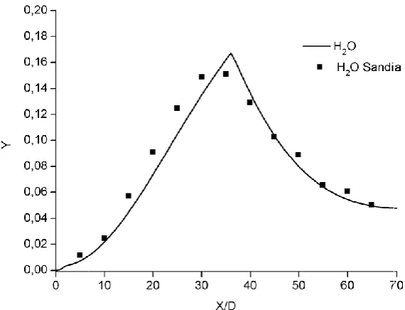
Figure 6. Comparison of the mixture fraction for

Figure 5: Local error over time interval.

Comparison of the mixture fraction for / jet with experiment.

jet with experiment.

(32c)

(32d)

(32e)

(32f)

(32g)

Figure 7. Mass fraction of

and considering , for

The local error estimation is given by

considering the norm as

The variables and are calculated using step

the increment for the step needs to be limited, which can be done by the following equation, agreeing with De Bortoli

It is also necessary that the values of the

step-small enough and, in case of rejection, the growth factor should be replaced by 1, instead of 10, in the next iteration.

Code verification

To evaluate the efficiency of the method used, some differential equation systems usually applied in numerical tests were selected. Robertson's (1966) model is one of the most well known problems for the analysis of stiff systems. The model describes the kinetics of an autocatalytic reaction whose reaction structure is given

where , and are the specific rates given by involved.

The model equation can be written as

14015 Régis S. de Quadros

Mass fraction of along the burner centerline.

and .

are calculated using step-size and , respectively. To avoid divergence during the iterative process the increment for the step needs to be limited, which can be done by the following equation, agreeing with De Bortoli

-size be limited by maximum and minimum values. The initial time increment must be rejection, the growth factor should be replaced by 1, instead of 10, in the next iteration.

of the method used, some differential equation systems usually applied in numerical tests were selected. model is one of the most well known problems for the analysis of stiff systems. The model describes the kinetics of an autocatalytic reaction whose reaction structure is given in.

are the specific rates given by , and and

Régis S. de Quadros et al.Asymptotic analysis of stoichiometric hydrogen-air flames

(33)

(34)

, respectively. To avoid divergence during the iterative process the increment for the step needs to be limited, which can be done by the following equation, agreeing with De Bortoli (2015):

(35)

size be limited by maximum and minimum values. The initial time increment must be rejection, the growth factor should be replaced by 1, instead of 10, in the next iteration.

of the method used, some differential equation systems usually applied in numerical tests were selected. model is one of the most well known problems for the analysis of stiff systems. The model describes the kinetics of

(36)

and , and are the species

(37a)

(37b)

(37c)

The integration interval used was with the initial conditions:

(38)

The points obtained from the integration developed by Silva (2013), using the Modified Extended Backward Differentiation Formulae (MEBDF), are shown in figures 1, 2 and 3 by squares. The stars corresponds to results obtained by Nagy et al. (2014) using MATLAB and the continuous line shows the results of fourth order Rosenbrock method.

RESULTS AND DISCUSSION

To obtain the behavior of the species concentration in relation to time, the system of reactive equations was solved by the fourth order Rosenbrock method with four stages and an adaptive control for the time-step. The numerical method was implemented in Fortran language. A tolerance for error = 10 was assumed. Figure 4 shows the results and Figure 5 shows the local error. As no experimental data for comparison of molar concentration of hydrogen was found in the literature, in the following the mixture fraction was compared to experimental values obtained from the researches of the Sandia National Laboratory (2010). The result for the mixture fraction ( ), shown in Figure 6, indicates the decay of the centerline velocity with downstream distance from the entrance. Based on the Burke-Schumann analytical solution (Warnatz et al 2006) and the equations presented by Lorenzetti et al (2010), the mass fraction of along the burner centerline is presented. The nitrogen acts as an inert, not affecting the jet diffusion flame. The result, shown in Figure 7, is satisfactory, despite the use of a simple model. The results obtained for the mixture fraction can now be compared with those of Lorenzetti et al (2010), and with the experimental data of Sandia National Laboratories (2010). The comparison is shown in Table 2. In some intervals, the values obtained are now closer to the experimental ones, as seen at / between 10 to 20 and 40 to 45, for example.

REFERENCES

Bui, T.D. 1977. On a L-stable method for stiff differential equations, Information Processing Letters, Vol. 6, No. 5, pp. 158-161. Bui, T.D. 1979a. A note on the Rosenbrock procedure, Mathematics of Computation, Vol. 33, No. 147, pp. 971-975.

Bui, T. D.; Bui, T. R. 1979b. Numerical methods for extremely stiff systems of ordinary differential equations, Applied

Mathematical Modelling, Vol. 3, No. 5, pp. 355-358.

Bui, T. D. 1979c. Some A-stable and L-stable methods for the numerical integration of stiff ordinary differential equations, Journal of the ACM (JACM), Vol. 26, No. 3, pp. 483-493.

Butcher, J. C. 1964. Implicit Runge-Kutta processes, Mathematics of Computation, Vol. 18, No. 85, p. 50-64.

Chamousis, R. 2009. Hydrogen: Fuel of the future, San Joaquin Valley, USA: UC Merced.

De Bortoli, A.L. and Andreis, G.S.L. 2012. Asymptotic analysis for coupled hydrogen, carbon monoxide, methanol and ethanol reduced kinetic mechanisms, Lat. Am. Appl. Res., Vol. 42, No. 3, pp 299-304.

De Bortoli, A.L.; Andreis, G.S.L.; Pereira, F. 2015. Modeling and Simulation of Reactive Flows. Elsevier.

Hairer, E.; Norsett, S. P.; Wanner, G. 1987. Solving ordinary di erential equations I: Nonsti problems. Springer.

Lambert, J.D. 1991. Numerical methods for ordinary differential systems: the initial value problem. John Wiley & Sons, Inc. Lorenzetti, G.S.; Vaz, F.A.; De Bortoli, A.L. 2010. An analytical solution for hydrogen/nitrogen jet diffusion flames, Mecánica

Computacional., No. 29, pp 2399-2405.

Marinov, N.M. 1999. A detailed chemical kinetic model for high temperature ethanol oxidation, Int. J. Chem. Kint., No. 31, pp 183-220.

Nagy, A. L.; Tóth, J.; Papp, D. 2014. Reaction Kinetics: Exercises, Programs and Theorems, Mathematical and Computational Chemistry.

Peters, N. 1992. Fifteen Lectures on Laminar and Turbulent Combustion, Ercoftac Summer School, Aachen, Germany.

Peters, N. 1988. Systematic reduction of flame kinetics - Principles and details, Dynamics of reactive systems. Part 1: Flames, pp 67– 86.

Robertson, H. H. 1966. The solution of a set of reaction rate equations, Numerical Analysis: an introduction, pp. 178-182.

Rosenbrock, H. H. 1963. Some general implicit processes for the numerical solution of differential equations. The Computer

Journal, Vol. 5, No. 4, pp. 329-330.

Sandia National Laboratories 2010. H2/N2 jet diffusion flame(H3), Re=10000.

Silva, D.V.A. 2013. Aprimoramento de Métodos Numéricos para a Integração Numérica de Sistemas Algébrico-Diferenciais.

MSc Thesis in Chemical Engineering. Federal University of Rio de Janeiro. Turns, S.R. 2000. An Introduction to Combustion. 2nd Ed. Boston: McGraw Hill.

Warnatz, J.; Maas, U.; Dibble, R. 2006. Combustion: Physical and Chemical Fundamentals, Modeling and Simulation, Experiments, Pollutant Formation. 4th Ed. Boston: McGraw Hill.