BIROn - Birkbeck Institutional Research Online
Skene, S.S. and Kenward, M.G. (2010) The analysis of very small samples of
repeated measurements II: a modified box correction. Statistics in Medicine
29 (27), pp. 2838-2856. ISSN 0277-6715.
Downloaded from:
Usage Guidelines:
Please refer to usage guidelines at or alternatively
The analysis of very small samples of repeated measurements
II: A modified Box correction
Simon S. Skenea∗† and Michael G. Kenwardb
There is a need for appropriate methods for the analysis of very small samples of continuous repeated measurements. A key feature of such analyses is the role played by the covariance matrix of the repeated observations. When subjects are few it can be difficult to assess the fit of parsimonious structures for this matrix, while the use of an unstructured form may lead to a serious lack of power. The Kenward-Roger adjustment is now widely adopted as a means of providing an appropriate inferences in small samples, but does not perform adequately in very small samples. Adjusted tests based on the empirical sandwich estimator can be constructed that have good nominal properties, but are seriously underpowered. Further, when such data are incomplete, or unbalanced, or non-saturated mean models are used, exact distributional results do not exist that justify analyses with any sample size. In this paper, a modification of Box’s correction applied to a linear model based F-statistic is developed for such small sample settings and is shown to have both the required nominal properties and acceptable power across a range of settings for repeated measurements.
Keywords: ANOVA; Box correction; covariance matrix; linear model; repeated measures; Scheff´es method; small samples
1. Introduction
The preceding companion paper to this [1] highlights the need for appropriate methods for the analysis of repeated measurements when the sample size is very small. In particular, deficiencies in conventional approaches to inference from such samples are highlighted where data are unbalanced or incomplete. It is shown that hypothesis tests based on conventional Wald type procedures do not approximate their nominal properties sufficiently well. This is the case with the Kenward-Roger adjustment [2, 3], which is implemented inSAS PROC MIXED[4] and accounts for both bias and variability in the estimated covariance matrix of the fixed effects by adoption of a scaled F-statistic and an adjustment to the denominator degrees of freedom. Also considered is the empirical sandwich estimator from the generalized estimating equations (GEE) approach for categorical data, which uses ordinary least squares
a
Department of Economics, Mathematics and Statistics, Birkbeck, London, UK.
b
Department of Medical Statistics, London School of Hygiene and Tropical Medicine, London, UK.
∗Correspondence to: Simon S. Skene, Department of Economics, Mathematics and Statistics, Birkbeck,
University of London, Malet Street, London WC1E 7HX, UK.
estimates for the fixed effects and adjusts their standard errors to reflect the observed de-pendencies in the data. Such a procedure is known to have poor small sample properties, but an adjusted Wald test due to Pan and Wall [5] can be generalised to allow testing of any general linear hypothesis involving fixed effects. When combined with a bias adjustment (Mancl and DeRouen [6]), the resulting statistic is seen to achieve adequate control over the type 1 error rate, but has very poor power in comparison to the Kenward-Roger adjusted statistic (when the latter provides a valid comparator). In this paper we consider further the need for an appropriate general approach, which will be applicable across a range of settings for repeated measures data where the sample size is very small.
The problems in the methods listed above all stem from the same source: the lack of infor-mation in the data on the covariance structure of the repeated measurements. In certain balanced settings with saturated mean models the covariance structure does not influence the parameter estimates which are then identical to those obtained from ordinary least squares. In such circumstances the Kenward-Roger adjustment recovers exact Hotelling’sT2 and hi-erarchical ANOVA F-tests which do not require small sample approximation. Moving away from such special cases, such as with missing data or with non-saturated models, leads to serious departures from the nominal properties of inference procedures in very small samples. It is clear from this that removing the estimated covariance structure from the estimation of the regression parameters leads to an improvement in the small sample behaviour of in-ferences. In such cases, the estimated covariance structure is not used in the estimation of the mean parameters, but is necessary for estimates of their precision. This control is seen to deteriorate where the covariance structure enters the estimation step, and is worse still in situations which are unbalanced. This suggests the use of ordinary least squares more widely in such settings, with subsequent correction of the measure of precision using a sand-wich (also termed empirical or robust) estimate of the covariance matrix of the estimates. In the companion paper it was shown how such procedures, with appropriate small sample modification of the sandwich estimator, produce test statistics with good approximation to their nominal size. However, the need to estimate the covariance matrix of the repeated measurements as part of the sandwich estimator leads to very poor precision of this, with a consequent impact on the power of the associated tests. This was seen to be unacceptably poor in small sample settings.
develop the modification in Section 3. The properties of the corrections are explored in Section 4. In Section 5 we compare, through a series of simulation studies across a range of repeated measurement settings, the performance of the corrections with the procedures based on the Kenward-Roger adjustment and the adjusted sandwich estimator. Examples of the use of the modified Box correction are presented in Section 6, where it is also shown how Scheff´e’s method [11] for obtaining confidence intervals for individual contrasts can be adapted to allow for the modified Box-corrected statistic. Practical recommendations for the analysis of very small samples of repeated measurements are then made in the discussion of Section 7.
2. Box’s correction
We suppose that the data can be represented by a conventional multivariate Gaussian linear model [12]. Let yi (Ti × 1) be the response vector from the ith of n subjects, and it is
assumed that a common set of measurement times applies to all subjects, although not all may be observed for all subjects. The model has the following general form
yi ∼N (Xiβ;Σi), i= 1, . . . , n, (1)
forβ, (p×1), the vector of fixed effect parameters, Xi, (Ti×p), the design/covariate matrix,
andΣi the (Ti×Ti) covariance matrix for this subject. Depending on the setting, the
covari-ance matrix can in principle take many forms, including those induced by a random effects structure. Defining y= (y1, . . . ,yn)T,X = (X1, . . . ,Xn)T, setting Σ= block-diagonal{Σi}
we have the equivalent expression for the whole data set:
Y ∼N (Xβ;Σ). (2)
Now suppose that we wish to test the null hypothesis that celements ofβ are zero, but not under the model assumptions above, but rather assuming (wrongly) independent equally variable Gaussian errors. DefineXR (n×(r−c)) to be the design matrix for the model with
the terms to be tested removed, and set A =I−X(XTX)−1XT and B=X(XTX)−1XT
−
XR(XTRXTR)−1XTR. Then, using the extra sums of squares principle, the appropriate test
statistic for the null hypothesis under the independence assumptions is given by
F = n−r
c
yTBy
yTAy, (3)
which, if these assumptions held, would have a null Fc,n−r distribution. Under the more
general model (2), Box [7, 8] showed that ψ−1F has an approximate F
v1,v2 distribution, where the degrees of freedom and ψ are obtained as follows. The key approximation [13] is to treat the numerator and denominator quadratic forms as having independent scaled chi-squared distributions of the form,
Q=yTCy approx∼ gχ2
where the constant and degrees of freedom parameters g and h are chosen by matching the first and second moments. That is
gh = tr(CΣ)
2g2h = 2tr(CΣCΣ)
From this we get
ψ = (n−r)
c
tr(BΣ)
tr(AΣ) (5)
v1 = {
tr(BΣ)}2
tr{(BΣ)2} (6)
v2 = {
tr(AΣ)}2
tr{(AΣ)2} (7)
In practice, any consistent estimator ofΣ= V(y), may be used to compute the adjusted F-distribution parameters. Jones and Keward [14] suggest the use of the ordinary least squares (OLS) covariance estimate is in keeping with the spirit of this approach. However, for data which are unbalanced or have missing values, so that the OLS and restricted maximum likelihood (REML) estimates do not coincide, it may be more practical to simply adopt the unstructured REML estimate, which is widely implemented in existing software. In cases where an unstructured REML estimate cannot be computed (as can occur, for example, where there are too many measurements on too few subjects), Σ may be taken to be the most complex covariance structure that the data will support, such as a (high order) antede-pendence structure. An advantage of this method is that it does not require a non-singular estimate of the covariance structure, so that, in such cases, it is possible to proceed using an ‘empirical’ estimator such as the sample covariance matrix.
In simulations (see below) Box’s correction can be shown to be conservative, giving excessive control over the type 1 error rate and resulting in test sizes well below the nominal rate, and so a modification to this correction is proposed.
3. A modified Box correction
Rather than approximating the distribution of the quadratic form in the F-statistic (3)
Q1 Q2
= y
TBy
yTAy
as a ratio of independent scaled chi-squared distributions, we instead approximate it directly by a scaled F-distribution, λFv1,v2, and match the first two moments of this. These can be obtained using the the ‘delta’ method (see, for example, Stuart and Ord [15]), from which we obtain
E
Q1 Q2
≈ E(Q1)
E(Q2)
and Var Q1 Q2
= {E(Q1)} 2
{E(Q2)}2
Var(Q1)
{E(Q1)}2
+ Var(Q2)
{E(Q2)}2 −
2Cov(Q1, Q2) E(Q1)E(Q2)
(9)
Assuming, as in the Box correction, that the numerator and denominator terms in the F -statistic are independent, so that Cov(Q1, Q2) = 0, we have, equating these moments with those of the scaled F-distribution
1
λ
tr(BΣ) tr(AΣ) =
v2 v2−2
(10)
and,
1
λ2
{tr(BΣ)}2
{tr(AΣ)}2
2tr{(BΣ) 2}
{tr(BΣ)}2 + 2
tr{(AΣ)2}
{tr(AΣ)}2
= 2v
2
2(v2+v1−2) v1(v2−2)2(v2−4)
(11)
Fixing v1 =c, the dimension of the test (similarly to the Kenward-Roger and small-sample sandwich adjustments), we can use these final two equations to obtain expressions for the scale factorλand the denominator degrees of freedomv2 for our approximating distribution. This gives us
F = (n−r)
c
yTBy yTAy
approx
∼ λFc,v2 (12)
where,
λ = (n−r)
c
v2−2 v2
tr(BΣ)
tr(AΣ) (13)
v2 =
c(4V + 1)−2
cV−1 (14)
and,
V =
tr{(BΣ)2}
{tr(BΣ)}2 +
tr{(AΣ)2}
{tr(AΣ)}2
(15)
Results from simulations showing the performance of this statistic across a range of settings for repeated measurements will be shown in Section 5. A further modification was considered using second order deviations about the mean in (8). That is, taking
E
yTBy yTAy
≈ tr(tr(BΣAΣ))
1 + 2tr{(AΣ) 2}
{tr(AΣ)}2 −2
tr(AΣBΣ) tr(AΣ)tr(BΣ)
(16)
4. Properties of the Box corrections
It is worth noting that under the assumption of independence, Box’s original correction recovers the ANOVAF-statistic exactly, whereas the modified correction does not, although the disparity is of small order. Although it is desirable to have a statistic which recovers the exact test in appropriate circumstances, such circumstances are unlikely to arise in practice in the context of repeated measurements.
It is also useful to consider how such corrections behave under the assumption of ‘compound symmetry’, and the relationship between this approach and repeated measures ANOVA. The latter approach was often adopted for ‘practical’ analyses before modern computing power allowed widespread access to the multivariate general linear model, which is now more commonly used for such data. See, for example, [16] for an outline to this approach, and [17] for more detail.
The general formulation is to treat ‘time’ (occasions of measurement) as an additional within-subjects factor, and to model the jth measurement on the ith subject as
yij =µij +bi+eij (17)
where µij are suitably specified fixed effects, bi ∼ N(0, σ2
b) are random (individual specific)
subject effects, and eij ∼N(0, σ2) are the usual error terms.
Two sources of variation, between-subjects and within-subjects, lead to a compound symme-try covariance structure for the repeated measurements, with a constant variance, σ2
b +σ2,
on the diagonal and a constant covariance off the diagonal, and hence a constant correlation between any pair of repeated measurements on the same subject, given by the intra-class correlation
ρ= σ 2 b σ2
b +σ2
(18)
Such an approach is appropriate when supported by randomization, such as in a randomised block, or split-plot, design, where the subjects are considered as blocks or main-plots re-spectively, and in extended examples involving more error strata, [18, 19]. However, this approach is not appropriate for the majority of repeated measurements studies because time cannot be randomized. Also, departures from constant correlation and constant variance are often, although not invariably, observed [12].
in general for such a model to be appropriate it is necessary only for the within-subjects covariance matrix to comply with the assumption of sphericity. This is a less restrictive condition than compound symmetry, since sphericity requires only that the variance of dif-ferences in a within-subjects design are equal across all groups. The Greenhouse and Geisser correction uses
F approx∼ Fǫ(p−1),ǫ(m−g)(p−1) (19)
wherep is the number of repeated measurements on a subject,m is the number of subjects, andg is the number of treatment groups. Adjusted tests usingǫdefined by both Greenhouse and Geisser and Huynh and Feldt are widely implemented in software packages.
Using the Box correction of Section 2, under the assumption of compound symmetry, we find
ψ = σ 2
σ2 b +σ2
= 1−ρ (20)
That is, the Box correction adjusts the one-way ANOVA F-statistic for ‘treatments’ to that which would be obtained from the (more restrictive) two-way setting, using ‘time’ as the other factor. This is equivalent to using an (unadjusted) Wald statistic for the regression parameters in a multivariate linear model with a compound symmetry covariance structure. However, although the numerator degrees of freedom are fixed, the denominator degrees of freedom are lower than from their two-way counterpart, since we are accounting for departures from independence. A similar relationship is found with the modified Box correction under compound symmetry.
In the context of very small samples of repeated measurements, the one-way ANOVA ap-proach with a suitable correction is preferred, since it is more widely applicable across a range of settings. The Greenhouse and Geisser approach, based on the split-plot design, is simply too restrictive to be of use generally, since it requires complete and balanced data and would not, for example, accommodate missing data or cross-over designs.
5. Simulation studies
To investigate the properties of the Box corrections it is appropriate to consider their use over a range of settings for repeated measurements. Consideration is given to the following study designs based on the simple repeated measurement and cross-over designs used to assess the existing repeated measurements methods in [1]. These simulations accommodate both a range of numbers of time points (T) and subjects (n), and include data arising from a wider variety of plausible non-stationary covariance structures. The extended simulation designs are detailed below. For the simple repeated measures designs, we have
(A′) A simple repeated measures experiment, with n subjects randomly allocated to two
treatment groups (of equal size), and a response recorded for each subject at each of
Table I. A cross-over design for nine treatments (A, B, C, D, E, F, G, H, I).
Period
Subject 1 2 3 4 5 6 7 8 9
1 A B C D E F G H I
2 B D A F C I H G E
3 C F E G D B I A H
4 D G F I B H E C A
5 E A I C H D F B G
6 F H B E I G A D C
7 G I D H F A C E B
8 H C G B A E D I F
9 I E H A G C B F D
10 I H G F E D C B A
11 E G H I C F A D B
12 H A I B D G E F C
13 A C E H B I F G D
14 G B F D H C I A E
15 C D A G I E B H F
16 B E C A F H D I G
17 F I D E A B G C H
18 D F B C G A H E I
(B′) As design (A′), but with missing values. An equal number of subjects in each treatment
group drop out at some random time following the first observation.
(C′) A five treatment-five period cross-over trial, with n = 10 and 20 subjects allocated
randomly to treatments according to Table I of [1], using a pair of Williams’ squares.
(D) A nine treatment-nine period cross-over trial, with n = 18 and 36 subjects allocated randomly to treatments according to Table I of this paper.
In designs (A′) and (B′), we consider T = 5 time points with n = 10 and 20 subjects, and
T = 10 time points with n = 20 and 40 subjects. Additionally, in design (B′), the numbers
of subjects allowed to drop out are given in Table II, below. For the extended simulations involving additional subjects in the cross-over designs (n= 20 in design (C′), and n= 36 in
design (D)), the allocation tables are simply repeated.
Table II. Number of drop out subjects in extended study design (B′).
Number of measurements Number of subjects Number of subjects
per subject (T) (n) to drop out
5 10 2
20 4
10 20 4
40 8
and no treatment effect in designs (C) and (D). Two underlying stationary covariance struc-tures, compound symmetry and AR1 (high correlation) are considered, together with three non-stationary structures, heterogeneous compound symmetry, heterogeneous AR1 and first order independence. For each of the non-stationary structures, variances are restricted so that they differ by no more than a factor of 10 over the range of the measurement times. These structures are shown in the Appendix.
Results from the extended simulations of study designs (A′) and (B′) are shown in Tables
III and IV respectively. The results of simulations concerning study designs (C′) and (D)
are shown in Table V.
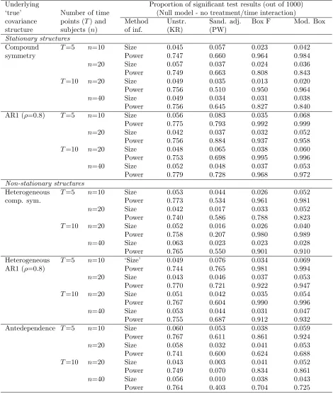
ForT = 5 time points in design (A′), we see that as the number of subjects rises from 10 to
20, the power of the tests using the Box corrections is above that of the KR adjusted Wald test for data arising from the stationary covariance structures. However, for data arising from the non-stationary structures, the increase in power is generally lower in comparison to the level attained by the KR adjusted test. This is particularly noticeable for the data arising from the antedependence structure, which is furthest from the univariate linear model assumptions of independence and homogeneity of variance. This is as we might expect, the performance of the KR adjusted test improving as the sample size increases, and the Box corrections performing comparatively less well for large departures from independence. A similar pattern is observed in design (B’), although the loss of power relative to the KR adjusted Wald test is more apparent for increased sample sizes where we have missing values.
As the number of time points increases to T = 10, the loss in power of the Box corrections relative to the KR adjusted test is less marked. That is, as the number of subjects and time points is increased in the balanced and complete data setting of design (A′), the modified
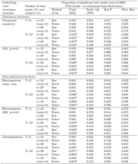
Box correction appears to hold its own against the KR adjusted Wald test. For design (B′),
where the missing values introduce imbalance, the KR adjustments no longer give an exact Hotelling T2 test, and must be calculated individually for each data set. For the (10×10) matrices necessitated by considering T = 10 time points, this is too expensive in terms of available computational time for such a practical study. In order to provide a comparison, the KR adjusted test results in Table IV have been estimated in each case using the ‘known’ underlying covariance structure and an average number of observations. This gives a measure of the best that could be achieved using the KR method, that is, an upper bound on its performance. The estimated results are marked with an asterisk in the table. Throughout Table IV, the KR adjustment is seen to give a test statistic with inflated size (for bothT = 5 and 10 time points), although this size is seen to approach the nominal level of 5% as the number of subjects increases.
In the extended simulations of study designs (A′) and (B′) tests involving the adjusted
Table III. Summary of results from 1000 simulations of extended study design (A′).
Underlying Proportion of significant test results (out of 1000)
‘true’ Number of time (Null model - no treatment/time interaction)
covariance points (T) and Method Unstr. Sand. adj. Box F Mod. Box
structure subjects (n) of inf. (KR) (PW)
Stationary structures
Compound T=5 n=10 Size 0.045 0.057 0.023 0.042
symmetry Power 0.747 0.660 0.964 0.984
n=20 Size 0.057 0.037 0.024 0.036
Power 0.749 0.663 0.808 0.843
T=10 n=20 Size 0.049 0.035 0.013 0.020
Power 0.756 0.510 0.950 0.964
n=40 Size 0.049 0.034 0.031 0.038
Power 0.756 0.645 0.827 0.840
AR1 (ρ=0.8) T=5 n=10 Size 0.056 0.083 0.035 0.068
Power 0.775 0.793 0.992 0.999
n=20 Size 0.042 0.037 0.032 0.052
Power 0.756 0.884 0.937 0.958
T=10 n=20 Size 0.048 0.065 0.038 0.060
Power 0.753 0.698 0.995 0.996
n=40 Size 0.052 0.048 0.037 0.053
Power 0.779 0.728 0.968 0.972
Non-stationary structures
Heterogeneous T=5 n=10 Size 0.053 0.044 0.026 0.052
comp. sym. Power 0.773 0.534 0.961 0.981
n=20 Size 0.042 0.017 0.033 0.052
Power 0.740 0.586 0.788 0.823
T=10 n=20 Size 0.052 0.016 0.026 0.040
Power 0.758 0.207 0.980 0.989
n=40 Size 0.063 0.023 0.023 0.028
Power 0.765 0.550 0.901 0.910
Heterogeneous T=5 n=10 ‘Size’ 0.049 0.076 0.034 0.069
AR1 (ρ=0.8) Power 0.744 0.765 0.981 0.994
n=20 Size 0.043 0.046 0.037 0.053
Power 0.770 0.721 0.922 0.947
T=10 n=20 Size 0.051 0.042 0.035 0.054
Power 0.767 0.604 0.990 0.996
n=40 Size 0.053 0.044 0.031 0.047
Power 0.755 0.687 0.912 0.932
Antedependence T=5 n=10 Size 0.060 0.053 0.038 0.059
Power 0.767 0.611 0.861 0.924
n=20 Size 0.058 0.032 0.041 0.053
Power 0.741 0.600 0.624 0.688
T=10 n=20 Size 0.043 0.003 0.041 0.052
Power 0.749 0.070 0.834 0.861
n=40 Size 0.056 0.010 0.038 0.043
Power 0.764 0.403 0.704 0.725
Table IV. Summary of results from 1000 simulations of extended study design (B′).
Underlying Proportion of significant test results (out of 1000)
‘true’ Number of time (Null model - no treatment/time interaction)
covariance points (T) and Method Unstr. Sand. adj. Box F Mod. Box
structure subjects (n) of inf. (KR) (PW)
Stationary structures
Compound T=5 n=10 Size 0.074 0.051 0.017 0.040
symmetry (miss=2) Power 0.632 0.523 0.882 0.937
n=20 Size 0.059 0.036 0.041 0.050
(miss=4) Power 0.644 0.505 0.733 0.772
T=10 n=20 Size 0.053* 0.050 0.012 0.023
(miss=4) Power 0.624* 0.361 0.857 0.890
n=40 Size 0.057* 0.038 0.046 0.052
(miss=8) Power 0.624* 0.449 0.610 0.643
AR1 (ρ=0.8) T=5 n=10 Size 0.078 0.064 0.024 0.061
(miss=2) Power 0.637 0.677 0.966 0.989
n=20 Size 0.067 0.050 0.052 0.067
(miss=4) Power 0.662 0.586 0.869 0.900
T=10 n=20 Size 0.068* 0.096 0.036 0.068
(miss=4) Power 0.645* 0.618 0.993 0.995
n=40 Size 0.062* 0.040 0.054 0.070
(miss=8) Power 0.674* 0.614 0.925 0.944
Non-stationary structures
Heterogeneous T=5 n=10 Size 0.084 0.056 0.019 0.042
comp. sym. (miss=2) Power 0.609 0.412 0.843 0.927
n=20 Size 0.054 0.032 0.043 0.059
(miss=4) Power 0.634 0.439 0.681 0.739
T=10 n=20 Size 0.062* 0.025 0.022 0.037
(miss=4) Power 0.627* 0.162 0.910 0.939
n=40 Size 0.063* 0.020 0.030 0.038
(miss=8) Power 0.667* 0.318 0.796 0.810
Heterogeneous T=5 n=10 Size 0.083 0.066 0.031 0.072
AR1 (ρ=0.8) (miss=2) Power 0.631 0.578 0.914 0.975
n=20 Size 0.048 0.025 0.052 0.070
(miss=4) Power 0.683 0.562 0.836 0.884
T=10 n=20 Size 0.048* 0.049 0.048 0.075
(miss=4) Power 0.602* 0.413 0.948 0.974
n=40 Size 0.058* 0.038 0.042 0.054
(miss=8) Power 0.658* 0.505 0.851 0.894
Antedependence T=5 n=10 Size 0.065 0.042 0.038 0.072
(miss=2) Power 0.664 0.494 0.748 0.862
n=20 Size 0.054 0.028 0.040 0.057
(miss=4) Power 0.658 0.472 0.558 0.634
T=10 n=20 Size 0.071* 0.000 0.034 0.049
(miss=4) Power 0.604* 0.040 0.767 0.813
n=40 Size 0.048* 0.005 0.036 0.043
(miss=8) Power 0.654* 0.174 0.603 0.628
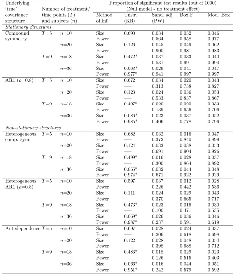
Table V. Summary of results from 1000 simulations of extended study designs (C′)
and (D).
Underlying Proportion of significant test results (out of 1000)
‘true’ Number of treatment/ (Null model - no treatment effect)
covariance time points (T) Method Unstr. Sand. adj. Box F Mod. Box
structure and subjects (n) of Inf. (KR) (PW)
Stationary Structures
Compound T=5 n=10 Size 0.690 0.034 0.032 0.046
symmetry Power —– 0.564 0.958 0.977
n=20 Size 0.126 0.045 0.049 0.062
Power —– 0.900 0.981 0.983
T=9 n=18 Size 0.472* 0.037 0.033 0.040
Power —– 0.531 0.991 0.994
n=36 Size 0.063* 0.029 0.041 0.047
Power 0.977* 0.941 0.997 0.997
AR1 (ρ=0.8) T=5 n=10 Size 0.672 0.034 0.020 0.043
Power —– 0.313 0.738 0.827
n=20 Size 0.123 0.024 0.036 0.053
Power —– 0.533 0.837 0.867
T=9 n=18 Size 0.497* 0.020 0.020 0.033
Power —– 0.139 0.656 0.706
n=36 Size 0.086* 0.023 0.037 0.052
Power 0.985* 0.406 0.778 0.796
Non-stationary structures
Heterogeneous T=5 n=10 Size 0.682 0.032 0.016 0.047
comp. sym. Power —– 0.372 0.840 0.899
n=20 Size 0.124 0.033 0.038 0.053
Power —– 0.691 0.904 0.926
T=9 n=18 Size 0.499* 0.016 0.028 0.037
Power —– 0.300 0.864 0.892
n=36 Size 0.065* 0.032 0.044 0.048
Power 0.974* 0.671 0.922 0.929
Heterogeneous T=5 n=10 Size 0.597 0.037 0.012 0.028
AR1 (ρ=0.8) Power —– 0.226 0.442 0.536
n=20 Size 0.111 0.024 0.029 0.043
Power —– 0.370 0.665 0.717
T=9 n=18 Size 0.473* 0.023 0.016 0.030
Power —– 0.100 0.471 0.535
n=36 Size 0.069* 0.026 0.036 0.046
Power 0.987* 0.237 0.591 0.619
AntedependenceT=5 n=10 Size 0.697 0.028 0.024 0.037
Power —– 0.206 0.618 0.698
n=20 Size 0.122 0.028 0.048 0.054
Power —– 0.398 0.688 0.712
T=9 n=18 Size 0.483* 0.018 0.029 0.023
Power —– 0.126 0.515 0.403
n=36 Size 0.066* 0.016 0.044 0.051
Power 0.951* 0.242 0.579 0.592
resulting in invalid (negative) estimates for the denominator degrees of freedom. In these instances, setting the numerator degrees of freedom to c, the dimensionality of the test, results in a single denominator degree of freedom test. These issues do not, however, reccur as the number of subjects increases, and the results for 10 time points and 20 subjects do not appear to be out of line.
Consider now the cross-over studies of designs (C′) and (D). For extended study design
(C′), based on the five treatment-five period design, we see that as the number of subjects
increases from 10 to 20, the test sizes using the KR adjustment are closer to the nominal level of 5%, but are too inflated for power to be considered. Power is compared for the adjusted sandwich estimator and the Box corrections for treatment differences which lead to comparable powers using the Wald statistic (with a KR adjustment and a ‘known’ covariance structure) of 100%. Again, the modified Box correction is seen to give a test with nominal properties and good power in comparison to the ‘true’ test.
Results from the simulations under study design (D) are obtained similarly, and the modified Box correction is again seen to give the better performance. As previously seen, the adjusted sandwich estimator results in invalid parameter estimates where the number of time points is increased and the number of subjects is small (n = 18), so that the denominator degrees of freedom of such tests are fixed at 1, close to the boundary.
In this setting, with an estimated (9 ×9) covariance structure, the KR adjustments are again computationally expensive in terms of 1000 individual simulations, so are estimated, for comparison purposes, using the ‘known’ structure to give an upper bound on the perfor-mance. (Again these estimated values are marked with an asterisk in the table). These show that the test size reduces towards nominal levels as the number of subjects increases, so that it may be appropriate to consider power. However, it is clear that these values cannot be achieved in practice.
6. Examples
Two examples are presented which illustrate the use of the modified Box correction in prac-tical analyses.
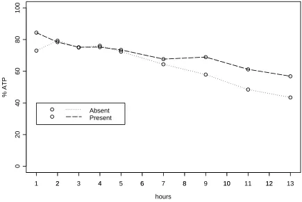
6.1. Cardiac enzyme in preserved dog hearts
hours
% ATP
2 4 6 8 10 12
0
20
40
60
80
100
1 2 3 4 5 6 7 8 9 10 11 12 13
[image:15.595.80.515.129.420.2]Absent Present
Figure 1. Cardiac enzyme data: mean profiles.
shown as Figure 1 and the pooled within-groups sample covariance-correlation matrix as Table VI.
Treating these data as a simple repeated measures design, a test for a treatment by time interaction using the unstructured covariance matrix with a Kenward-Roger (KR) small sample adjustment is equivalent to an exact Hotelling T2 test. The upper panel of Table VII shows the results obtained from Wald tests using various covariance models and the modified Box correction. It can be seen that the test results differ according to the choice of structure. As the data are complete and balanced, the same mean estimates (by ordinary least squares) are obtained under each method, but they differ in their estimates of precision.
The exact HotellingT2test obtained using the unstructured covariance matrix indicates that there is insufficient evidence (at the 5% level) to reject the null hypothesis of no treatment by time interaction. This is confirmed by the modified Box corrected statistic, although in this instance the evidence is less marginal than that offered by the Hotelling T2 test.
Table VI. Sample covariance-correlation matrix for the cardiac enzyme data.
37.08 11.29 4.04 32.53 24.78 37.22 51.32 19.08 15.89 0.34 29.27 -3.52 12.80 7.64 10.02 18.66 8.14 -7.84
0.12 -0.11 33.08 -7.70 15.43 6.91 15.80 -11.43 30.00
0.47 0.21 -0.12 128.08 -27.86 6.51 58.84 19.38 -43.17
0.58 0.20 0.38 -0.35 48.85 46.33 33.20 24.45 53.01
0.57 0.17 0.11 0.05 0.62 114.22 86.48 44.59 61.27 0.78 0.32 0.25 0.48 0.44 0.75 117.38 51.39 48.76
0.30 0.14 -0.19 0.16 0.33 0.40 0.45 111.24 42.10
0.27 -0.15 0.54 -0.39 0.78 0.59 0.46 0.41 94.24
Variances on the diagonal with covariances above and correlations below.
Table VII. Cardiac enzyme data: comparison of results.
Num. Den.
Covariance structure df df F p
Complete data
Identity - independence 8 90 1.49 0.1713
Unstructured 8 3 8.73 0.0509
Compound symmetry 8 80 2.07 0.0485
AR1 8 73.8 1.24 0.2904
Mod. Box (λ= 0.59) 8 11.2 2.52 0.0774
With artificial dropout
Identity - independence 8 87 1.87 0.0753
Unstructured 8 1.6 88.63 0.0252
Compound symmetry 8 77.2 2.32 0.0274
AR1 8 12.2 1.51 0.1686
Mod. Box (λ= 0.66) 8 10.48 2.84 0.0591
mean parameters as well as their standard errors are dependent on the choice of covariance structure, we introduce an artificial dropout to this reduced data set. To achieve this, consider that the three final measurements are missing from one of the dog hearts which receives the preserving liquid from which component A is absent. Repeating the tests for a treatment/time interaction with this artificial dropout gives the results shown in the lower panel of Table VII.
Now the tests using the KR adjustment (with the identity, unstructured, and compound symmetry structures) are no longer exact, and so these results are less plausible given the performance of such tests in our simulations. There is a higher significance of an interaction using the unstructured form once the three observations from the ‘absent’ group are removed, but the test using the modified Box correction remains non-significant.
6.2. Electrocardiogram abnormalities in the guinea pig papillary muscle
As the second example, we present analysis of data published by Brammer [23] which illus-trated the need for methods specific to very small samples of repeated measurements.
These data comprise measurements taken from papillary muscles dissected from the right ventricles of each of just three guinea pigs’ hearts in two experiments. The purpose of the experiments was to determine whether the compounds are likely to cause electrocardiogram abnormalities. Brammer recognises that analysis from such small samples is unlikely to be definitive, but notes that such small samples are common in isolated tissue or organ experiments.
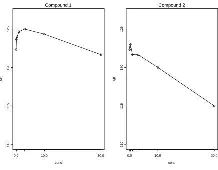
Since the isolated tissue assays from the guinea pigs deteriorate in time, there is a limited period in which to test different concentrations of the compounds on each muscle, so a control measure is followed by six increasing concentrations of the compound. In such an ascending dose design, the carryover effect is considered to be minimal in comparison to the current dose. Concentration and time are confounded, but a separate ‘control’ experiment with no compound present showed that there were no important changes over time. Five variables were measured, but we focus here on AP (amplitude of action potential). Mean profiles under each compound are shown in Figure 3.
These experiments can be considered as block designs, with concentration of compound as the treatment and tissue as the blocking factor, but the compound symmetry structure imposed by such a design may not be appropriate. Instead, Brammer treats the experiments as simple repeated measures designs with concentration as the time variable and tissue as the subject, and compares the resulting analyses from adopting various covariance models to account for the correlation between measurements on the same tissue (subject).
conc
AP
Compound 1
0.0 10.0 30.0
110
115
120
125
conc
AP
Compound 2
0.0 10.0 30.0
110
115
120
[image:18.595.82.519.90.431.2]125
Figure 2. GPPM data: mean profiles, compounds 1 and 2.
covariance models did not converge. Brammer compares those correlation structures that can be fitted by informal comparison of the (reduced) log-likelihoods and prefers an AR1 or heterogeneous AR1 model in each case over the more usual compound symmetry approach adopted for such experiments. However, the results of the simulations in [1] show that, for small samples, such methods are unreliable for choosing an appropriate structure.
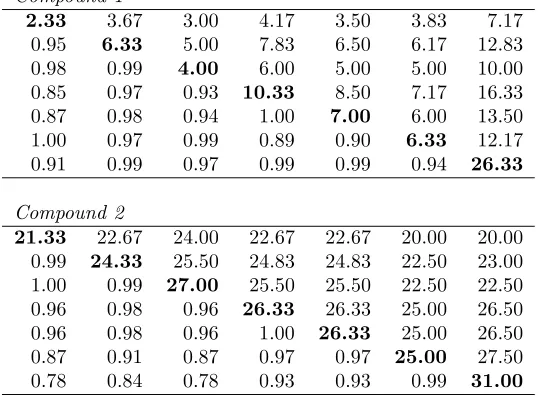
It is of interest to compare Brammer’s approach with that offered by the modified Box correction in this extreme small sample setting. Whilst the estimation method for the unstructured covariance model did not converge for either of the two experiments, it is possible to construct the (singular) sample covariance matrix directly in each case. The resulting estimates are shown in Table VIII below. While these matrices do not allow the construction of the usual Wald tests, which require invertible matrices, they can be used directly in the modified Box correction to allow the tests to reflect the observed dependencies in the data.
Table VIII. Sample covariance-correlation matrices for the GPPM data: compounds 1 and 2.
Compound 1
2.33 3.67 3.00 4.17 3.50 3.83 7.17
0.95 6.33 5.00 7.83 6.50 6.17 12.83
0.98 0.99 4.00 6.00 5.00 5.00 10.00
0.85 0.97 0.93 10.33 8.50 7.17 16.33
0.87 0.98 0.94 1.00 7.00 6.00 13.50
1.00 0.97 0.99 0.89 0.90 6.33 12.17
0.91 0.99 0.97 0.99 0.99 0.94 26.33
Compound 2
21.33 22.67 24.00 22.67 22.67 20.00 20.00 0.99 24.33 25.50 24.83 24.83 22.50 23.00 1.00 0.99 27.00 25.50 25.50 22.50 22.50 0.96 0.98 0.96 26.33 26.33 25.00 26.50 0.96 0.98 0.96 1.00 26.33 25.00 26.50 0.87 0.91 0.87 0.97 0.97 25.00 27.50 0.78 0.84 0.78 0.93 0.93 0.99 31.00
Variances on the diagonal with covariances above and correlations below.
measurement, a more appropriate method is suggested as follows.
1. Use the modified Box correction to test for an overall treatment (concentration) effect.
2. If significant, use Scheff´e’s method, in conjunction with the adjusted F-statistic, to test individual contrasts.
This approach ensures that the type 1 error rate for individual tests is controlled for mul-tiplicity of testing, as well as to departures from independence in the small sample setting for which the modified Box correction has been shown to be successful for the analysis of repeated measurements.
Scheff´e’s method [11] allows for the comparison of any or all possible contrasts between treatment means, ensuring that the type 1 error rate is at most α for any of the possible comparisons. It takes advantage of the union-intersection test properties of the ANOVA
F-statistic, by simultaneously considering all possible contrasts in the treatment means:
Γa =a1µ1 +a2µ2+. . .+arµr (21)
for anya=(a1, . . . , ar), withPai = 0. The corresponding contrasts in the treatment averages ¯
yi., are hence
Ca =a1y¯1.+a2y¯2.+. . .+aryr.¯ (22) and the standard error of this contrast is
SCa = v u u
tσˆ2
r
X
i=1 (a2
where ni is the number of observations of the ith treatment, and ˆσ2 is the mean squared error (MSE) of the data.
To use Scheff´e’s method with the modified Box corrected ANOVA statistic from (12) with (13)-(15), we have ˆσ2 = MSE =yTAy/(n
−r), and the critical value to whichCa should be compared is
Sα,a =SCa r
c
λFα;c,v2 (24)
so that a 100(1-α)% confidence interval for Ca is given by
Ca±Sα,a =Ca±SCa r
c
λFα;c,v2 (25)
An advantage of Scheff´e’s method is that it will always agree with the ANOVA F-test in the sense that if the F-test detects differences, then at least one Scheff´e test will detect a difference. Conversely, if the F-test does not detect any differences, then none of Scheff´e’s tests will. This is illustrated below using Brammer’s data.
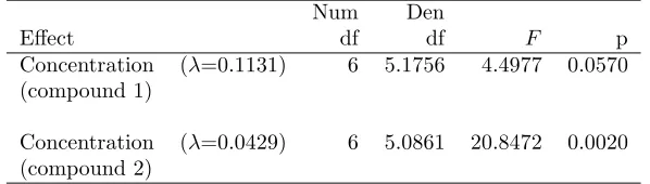
[image:20.595.157.456.429.514.2]We begin by considering the overall tests for a concentration effect, given in Table IX. The results show that there is only marginal evidence of a significant effect of concentration with compound 1, but that the evidence of a significant effect in compound 2 is much stronger.
Table IX. GPPM data: results using the modified Box correction.
Num Den
Effect df df F p
Concentration (λ=0.1131) 6 5.1756 4.4977 0.0570
(compound 1)
Concentration (λ=0.0429) 6 5.0861 20.8472 0.0020
(compound 2)
Table gives results of tests of overall treatment effect using the modified Box correction adopting thesingularsample covariance matrix.
Turning to the Scheff´e tests of individual contrasts (differences from control), we have, for compound 1, ˆσ2=8.9524, so that the standard error for the first, and actually all, the con-trasts is given by
SC1 = v u u
tˆσ2
7
X
i=1 (a2
i/ni) =
p
8.9524(1 + 1)/3 = 2.4430
and, since the 0.95-quantile of F(6,5.1756) is 4.8063, we find the 95% confidence interval for the first contrast is
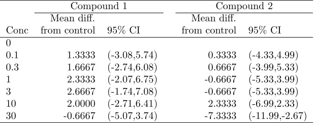
Table X. GPPM data: individual contrasts using Scheff´e’s method with the modified Box correction.
Compound 1 Compound 2
Mean diff. Mean diff.
Conc from control 95% CI from control 95% CI
0
0.1 1.3333 (-3.08,5.74) 0.3333 (-4.33,4.99)
0.3 1.6667 (-2.74,6.08) 0.6667 (-3.99,5.33)
1 2.3333 (-2.07,6.75) -0.6667 (-5.33,3.99)
3 2.6667 (-1.74,7.08) -0.6667 (-5.33,3.99)
10 2.0000 (-2.71,6.41) 2.3333 (-6.99,2.33)
30 -0.6667 (-5.07,3.74) -7.3333 (-11.99,-2.67)
Table gives Scheff´e confidence intervals for individual concentration differences from control using the modified Box statistics of Table IX.
Confidence intervals for the remaining contrasts are calculated similarly, (for compound 2, ˆ
σ2 = 25.9048). The results are shown in Table X.
As is expected, since the overall concentration effect was non-significant at the 5% level, none of the 95% confidence intervals for mean difference from control for compound 1 exclude zero. Of the contrasts with compound 2, only the final concentration is significantly different from control, 95% CI (-11.99, 2.67). (In fact this contrast is also significant at the 1% level, 99% CI (-14.14, -0.52)).
7. Discussion
The extensive simulation studies of Section 5 show that the modified Box correction results in a test with correct size which is more powerful than the other methods considered across a range of small sample settings for the analysis of repeated measurements. This is also seen to be the case in further simulations undertaken by the authors, for data arising from underlying covariance structures with low to medium correlation, such as the independence and AR1 (ρ = 0.2) structures used in the simulations of the companion paper. For such data, as might be expected, the Box corrections are most powerful, as we are closest in this setting to the underlying assumptions of the ANOVA statistic from which they originate.
subjects, but rather how it is used in inference. That is, where exactly such assumptions about the covariance structure enter the process. Further simulations (not presented) have shown no significant loss of power using the Box corrections where a common covariance structure is not assumed, such as when allowing the structure to change between treatment groups. However, convergence problems can arise in estimating the unstructured form using REML in this instance in the most extreme small sample settings.
The simulations confirm that Wald tests using an unstructured covariance matrix with the Kenward-Roger adjustment give inflated type 1 error rates where the data do not allow for exact tests, although the size of such tests does approach nominal levels as the sample size increases as we might expect. Where nominal properties are achieved, so that it is appropriate to consider power, we see that where the sample size (number of subjects) is small, tests using the Box corrections give greater power than the corresponding Wald tests. As the sample size increases the improvement in power from using the Box corrections over the KR adjustment diminishes as the underlying covariance structure moves further from independence, but the correction remains an effective method for inference.
The modified Box correction developed in Section 3 is preferred to Box’s original statistic which is conservative and hence less powerful. This method can, by suitable parameteriza-tion of the design matrix, be used to test any hypothesis involving fixed effects, based on their ordinary least squares estimates under the assumption of independence, and using any consistent estimator of the covariance matrix, such as that obtained from REML. It can be easily implemented using statistical software with minimal programming. Also, seen in the examples in Section 6 it is easily combined with Scheff´e’s method for simultaneous contrasts to examine questions of interest arising from significant tests, and providing appropriate control for multiple testing.
Appendix A
The following (5×5) and (10×10) symmetric matrices are used as the underlying covari-ance structures for the data generated in the simulations of extended designs (A′), (B′)and
(C′) used in the Section 5. The (9
A.1. Compound Symmetry σ2 1 +σ2
σ2
1 σ12+σ2 σ2
1 σ12 σ12+σ2 σ2
1 σ12 σ12 σ12+σ2 σ2
1 σ12 σ12 σ12 σ12+σ2 ..
. ... ... ... ... . ..
σ2
1 σ12 σ12 σ12 σ12 . . . σ12+σ2
with σ2
1 = 1 andσ2 = 1. We obtain the (5×5) and (10×10) matrices
2 1 2 1 1 2 1 1 1 2 1 1 1 1 2
and 2 1 2 1 1 2 1 1 1 2 1 1 1 1 2 1 1 1 1 1 2 1 1 1 1 1 1 2 1 1 1 1 1 1 1 2 1 1 1 1 1 1 1 1 2 1 1 1 1 1 1 1 1 1 2
A.2. AR1 σ2 1 ρ 1
ρ2 ρ 1 ρ3 ρ2 ρ 1 ρ4 ρ3 ρ2 ρ 1
... ... ... ... ... ...
ρ9 ρ8 ρ7 ρ6 ρ5 . . . ρ
with σ2 = 1 andρ= 0.8. We obtain the (5×5) and (10×10) matrices
1
0.8 1
0.64 0.8 1
0.512 0.64 0.8 1 0.4096 0.512 0.64 0.8 1
and 1
0.8 1
0.64 0.8 1
0.512 0.64 0.8 1
0.4096 0.512 0.64 0.8 1
0.3277 0.4096 0.512 0.64 0.8 1
0.2622 0.3277 0.4096 0.512 0.64 0.8 1 0.2098 0.2622 0.3277 0.4096 0.512 0.64 0.8 1 0.1678 0.2098 0.2622 0.3277 0.4096 0.512 0.64 0.8 1 0.1343 0.1678 0.2098 0.2622 0.3277 0.4096 0.512 0.64 0.8 1
A.3. Heterogeneous compound symmetry
σ2 1
σ2σ1ρ σ22
σ3σ1ρ σ3σ2ρ σ32
σ4σ1ρ σ4σ2ρ σ4σ3ρ σ42
σ5σ1ρ σ5σ2ρ σ5σ3ρ σ5σ4ρ σ52 ..
. ... ... ... ... . ..
σ10σ1ρ σ10σ2ρ σ10σ3ρ σ10σ4ρ σ10σ5ρ . . . σ102
For the (5×5) structure, we use ρ = 0.5, with σ2
1 = 1, σ22 = 2,σ32 = 3, σ42 = 4, and σ52 = 5, to obtain 1
0.7071 2
0.8660 1.2247 3
1.0000 1.4142 1.7321 4 1.1180 1.5811 1.9365 2.2361 5
For the (10×10) structure, we use ρ = 0.5, with σ2
σ2
6 = 6, σ27 = 7, σ28 = 8, σ92 = 9 and σ210= 10, to obtain
1
0.7071 2
0.8660 1.2247 3
1.0000 1.4142 1.7321 4
1.1180 1.5811 1.9365 2.2361 5
1.2247 1.7321 2.1213 2.4495 2.7386 6
1.3229 1.8708 2.2913 2.6458 2.9580 3.2404 7
1.4142 2.0000 2.4495 2.8284 3.1623 3.4641 3.7417 8
1.5000 2.1213 2.5981 3.0000 3.3541 3.6742 3.9686 4.2426 9
1.5811 0.2361 2.7386 3.1623 3.5355 3.8730 4.1833 4.4721 4.7434 10
A.4. Heterogeneous AR1
σ2 1
σ2σ1ρ σ22
σ3σ1ρ2 σ3σ2ρ σ32
σ4σ1ρ3 σ4σ2ρ2 σ4σ3ρ σ42
σ5σ1ρ4 σ5σ2ρ3 σ5σ3ρ2 σ5σ4ρ σ52 ..
. ... ... ... ... . ..
σ10σ1ρ9 σ10σ2ρ8 σ10σ3ρ7 σ10σ4ρ6 σ10σ5ρ5 . . . σ210
For the (5×5) structure, we use ρ = 0.8, with σ2
1 = 1, σ22 = 2,σ32 = 3, σ42 = 4, and σ52 = 5, to obtain 1
0.1314 2
1.1085 1.9596 3
1.0240 1.8102 2.7713 4 0.9159 1.6191 2.4787 3.5777 5
For the (10×10) structure, we use ρ = 0.8, with σ2
1 = 1, σ22 = 2, σ32 = 3, σ42 = 4, σ52 = 5, σ2
1
0.1314 2
1.1085 1.9596 3
1.0240 1.8102 2.7713 4
0.9159 1.6191 2.4787 3.5777 5
0.8026 1.4189 2.1722 3.1353 4.3818 6
0.6936 1.2261 1.8770 2.7092 3.7863 5.1846 7
0.5932 1.0486 1.6053 2.3170 3.2382 4.4341 5.9867 8
0.5033 0.8897 1.3621 1.9661 2.7477 3.7624 5.0798 6.7882 9
0.4244 0.7503 1.1487 1.6579 2.3170 3.1727 4.2837 5.7243 7.5895 10 A.5. Antedependence σ2 1
σ1σ2ρ1 σ22
σ1σ3ρ1ρ2 σ2σ3ρ2 σ32
σ1σ4ρ1ρ2ρ3 σ2σ4ρ2ρ3 σ3σ4ρ3 σ42 σ1σ5ρ1ρ2ρ3ρ4 σ2σ5ρ2ρ3ρ4 σ3σ5ρ3ρ4 σ4σ5ρ4 σ52
... . ..
σ1σ10ρ1ρ2ρ3ρ4ρ5ρ6ρ7ρ8ρ9 σ102
With σ2
1 = 1, σ22 = 2,σ32 = 3, σ42 = 4,σ52 = 5, ρ1 = 0.8, ρ2 = 0.6, ρ3 = 0.4, and ρ4 = 0.2, we have the (5×5) matrix
1
1.1314 2
0.8314 1.4697 3
0.3840 0.6788 1.3856 4 0.0859 0.1518 0.3098 0.8944 5
For the (10×10) structure, we use σ2
1 = 1,σ22 = 2,σ32 = 3, σ42 = 4, σ52 = 5,σ62 = 6, σ72 = 7, σ2
8 = 8, σ29 = 9 and σ102 = 10, with ρ1 = 0.8, ρ2 = 0.725, ρ3 = 0.65, ρ4 = 0.575, ρ5 = 0.5, ρ6 = 0.425, ρ7 = 0.35, ρ8= 0.275 and ρ9 = 0.2 to obtain
1
0.1314 2
1.0046 1.7759 3
0.7540 1.3329 2.2517 4
0.4847 1.8569 1.4475 2.5715 5
0.2655 0.4693 0.7928 1.4085 2.7386 6
0.1219 0.2154 0.3640 0.6466 1.2572 2.7543 7
0.0456 0.0806 0.1362 0.2419 0.4704 1.0306 2.6912 8
0.0133 0.0235 0.0397 0.0706 0.1372 0.3006 0.7640 2.3335 9
Acknowledgements
We are grateful to Professor Emmanuel Lessafre of the Catholic University of Leuven and to Dr Richard Brammer of Huntingdon Life Sciences for the Cardiac Enzyme and GPPM data respec-tively, which are used to illustrate our methods in Section 6. We are also grateful to the reviewers of this paper and the preceding companion paper for their comments and suggestions which have led to an improved work.
References
1. Skene SS, Kenward MG. The analysis of very small samples of repeated measurements. i. An adjusted sandwich estimator. Statistics in Medicine. DOI: 10.1002/sim.4073.
2. Kenward MG, Roger JH. Small sample inference for fixed effects from restricted maximum likelihood. Biometrics 1997; 53:983–997. DOI: 10.2307/2533558.
3. Kenward MG, Roger JH. An improved approximation to the precision of fixed effects from restricted maximum likelihood. Computational Statistics and Data Analysis, 2009; 53:2583– 2595. DOI: 10.1016/j.csda.2008.12.013.
4. SAS Institute Inc. 2004. SAS/STATR 9.1User’s Guide Cary, NC: SAS Institute Inc.
5. Pan W, Wall MM. Small-sample adjustments in using the sandwich variance estimator in gener-alized estimating equations.Statistics in Medicine2002;21:1429-1441. DOI: 10.1002/sim.1142.
6. Mancl LA, DeRouen TA. A covariance estimator for GEE with improved small-sample prop-erties.Biometrics 2001; 57:126-134. DOI: 10.1111/j.0006-341X.2001.00126.x.
7. Box GEP. Some theorems on quadratic forms applied in the study of analysis of variance prob-lems, i. effect of inequality of variance in one-way classification. The Annals of Mathematical Statistics 1954; 25:290–302. DOI: 10.1214/aoms/1177728786.
8. Box GEP. Some theorems on quadratic forms applied in the study of analysis of variance prob-lems, ii. effects of inequality of variance and of correlation between errors in two-way classifica-tion.The Annals of Mathematical Statistics1954;25:484–498. DOI: 10.1214/aoms/1177728717.
9. Bellavance F, Tardif S, Stephens MA. Tests for the analysis of variance of crossover designs with correlated errors.Biometrics 1996;52:607–612. DOI: 10.2307/2532899.
10. Chen, X, Wei L. A comparison of recent methods for the analysis of small sample cross-over studies.Statistics in Medicine 2003; 22:2821–2833. DOI: 10.1002/sim.1537.
11. Scheff´e H. A method for judging all contrasts in the analysis of variance. Biometrika 1953;
40:87–104. DOI: 10.1093/biomet/40.1-2.87.
13. Satterthwaite FE. Synthesis of Variance. Psychometrika 1941; 6:309–316. DOI: 10.1007/BF02288586.
14. Jones B, Kenward MG. Design and analysis of cross-over trials (2nd edn). Chapman and Hall/CRC, 2003.
15. Stuart A, Ord JK. Kendall’s advanced theory of statistics: vol 1. Distribution Theory (6th edn). Hodder Arnold, 1994.
16. Fitzmaurice GM, Laird NM, Ware JH. Applied Longitudinal Analysis Wiley, 2004.
17. Crowder MJ, Hand DJ.Analysis of Repeated Measures Chapman and Hall, 1990.
18. Nelder JA. The analysis of randomized experiments with orthogonal block structure. i. block structure and the null analysis of variance. Proceedings of the Royal Society of London. Series A, Mathematical and Physical Sciences 1965;283:147–162. DOI: 10.1098/rspa.1965.0012.
19. Nelder JA. The analysis of randomized experiments with orthogonal block structure. ii. treatment structure and the general analysis of variance. Proceedings of the Royal Soci-ety of London. Series A, Mathematical and Physical Sciences 1965; 283:163–178. DOI: 10.1098/rspa.1965.0013.
20. Geisser S, Greenhouse SW. An extension of Box’s results on the use of the F distribu-tion in multivariate analysis The Annals of Mathematical Statistics 1958; 29:885–891. DOI: 10.1214/aoms/1177706545.
21. Greenhouse SW, Geisser S. On methods in the analysis of profile data. Psychometrika 1959;
24:95–112. DOI: 10.1007/BF02289823.
22. Huynh H, Feldt LS. Estimation of the Box correction for degrees of freedom from sample data in randomized block and split-plot designs. Journal of Educational Statistics 1976; 1:69–82. DOI: 10.3102/10769986001001069.