A Soft Computing Approach to Dynamic Load Balancing in 3GPP LTE

35

A Soft Computing Approach to Dynamic Load Balancing

in 3GPP LTE

Aderemi A. Atayero

Covenant University, Ota, Nigeria

Matthew K. Luka

Covenant University, Ota, Nigeria

ABSTRACT

A major objective of the 3GPP LTE standard is the provision of high-speed data services. These services must be guaranteed under varying radio propagation conditions, to stochastically distributed mobile users. A necessity for determining and regulating the traffic load of eNodeBs naturally ensues. Load balancing is a self-optimization operation of self-organizing networks (SON). It aims at ensuring an equitable distribution of users in the network. This translates into better user satisfaction and a more efficient use of network resources. Several methods for load balancing have been proposed. Most of the algorithms are based on hard (traditional) computing which does not utilize the tolerance for precision of load balancing. This paper proposes the use of soft computing, precisely adaptive Neuro-fuzzy inference system (ANFIS) model for dynamic QoS aware load balancing in 3GPP LTE. The use of ANFIS offers learning capability of neural network and knowledge representation of fuzzy logic for a load balancing solution that is cost effective and closer to human intuition

Keywords

ANFIS, Soft computing, 3GPP LTE, Load balancing

1.

INTRODUCTION

Load balancing is a self-organizing function specified for the design of Long Term Evolution Radio Access Network (LTE RAN). The core objective of load balancing is to offset local load imbalance between neighbouring cells so as to improve the overall system capacity [1], [2]. Load balancing can be realized by optimizing the cell reselection/handover parameters such as hysteresis based on load imbalance between neighbouring eNodeBs. In addition to improving the overall system capacity, load balancing is of significant benefit to both network operators and subscribers. On the part of network operators, autonomous load balancing minimizes human intervention, which helps cut down both capital and operational cost as well as ensures that network resources are evenly used. On the other hand, the subscriber stands to get a better service satisfaction experience.

Several load-balancing techniques have been proposed in the literature [3, 4, 5]. All the methods proposed in these works and many other approaches use hard (traditional) computing which demands rigor, precision and certainty. However, precision and certainty carry a cost that should be leveraged by computation, reasoning and decision making (inference) wherever there is tolerance for imprecision and uncertainty [6]. Since the task of load balancing is ill-defined due to the unpredictable mobility of users, there exist a degree of uncertainty and imprecision that can be capitalized upon. Thus, the concept of soft computing proposed by LotfiZadeh [6] can be applied to load balancing. Soft computing which is a multi-disciplinary subject have been applied to a number of

productsranging from household devices to space-craft system. Some of the applications of soft computing in communication networks include: 1) the use of evolutionary computing to for channel assignment in cellular radio networks [7], use of genetic algorithm for design of communication networks [8] and the use of neural network for estimation of received power level in direct sequence code division multiple access [9]. A comprehensive review of the applications of soft computing in mobile and wireless networks is presented in [10].

This paper proposes the use of a soft computing technique that is based on the synergy of neural network and fuzzy logic for load balancing in the third Generation Partnership Project (3GPP) Long Term Evolution (LTE) radio access network.

2.

OVERVIEW OF SOFT COMPUTING

Soft computing is a class of computational intelligence tools and techniques shared by closely related disciplines such as genetic algorithms, belief calculus, artificial neural network, fuzzy logic and some machine learning methods like inductive reasoning. These computational tools can be used synergistically or independently; depending on the spectrum of the problem [11]. The primary objective of soft computing is the development of intelligent machines to address real life problems that are either too difficult or impossible to be modelled mathematically[12]. Soft computing aims to capitalize on uncertainty, approximation, imprecision and partial truth in order to mimic human intuition. Uncertainty implies one is not sure that the features of the model are the same as that of the entity. Also, imprecision means that the model features are not the same as the real ones but close to them. At its own end, approximation indicates that the model quantities are similar to the real ones but not the same. The Core disciplines of soft computing are Fuzzy Logic, Artificial Neural Networks and Genetic Algorithms. The combination of fuzzy logic and neurocomputing has the highest visibility [13]. Such systems called Neuro-fuzzy systems are very important for making inferences. To this end, an effective method called Adaptive Neuro-Fuzzy Inference System (ANFIS) was proposed in [14].

2.1 Fuzzy Logic

36 membership is matter of degree. In addition to fuzzy logic,

fuzzy sets have other branches such as fuzzy topology, fuzzy mathematical programming, fuzzy inference systems, fuzzy arithmetic and fuzzy data analysis.

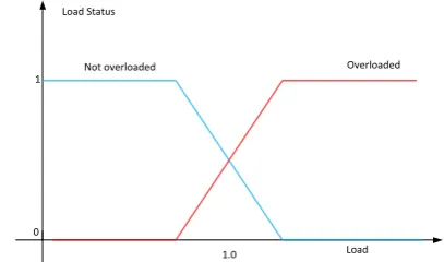
The concepts and reasoning modes underlining fuzzy logic makes it a suitable candidate for solving problems that require human intuition due to the absence of precise or accurate answer. For example, using traditional logic, the load condition of a cell in a mobile network can only be described as either overloaded or not overloaded. However, using fuzzy logic, one can specify the degrees of overload or otherwise of the cell with linguistic labels such as lightly loaded, normal, overloaded, heavily overloaded etc. In fig.1, the use of fuzzy logic to represent degree of truth is illustrated. A cell load of 0.8 belongs to both overloaded and not overloaded sets with a particular degree of membership. As the load increases, the membership grade within the overloaded set increases while the membership grade within the not overloaded set decreases.

1

0

1.0 Load Not overloaded Overloaded Load Status

Fig. 1 degree of truth representation using fuzzy logic

2.2 Artificial Neural Network

An Artificial Neural Network (ANN) is an information processing system that is modelled based on the performance characteristic of biological neural networks. It is made up of a large number of simple processing elements callednodes, units, cells, or neurons. Each node is connected to other nodes bymeans of directed communication links, each with an associated weight. Theweights represent information being used by the net to solve a problem [15]. ANN is characterized by 1) architecture (the pattern of connections between the cells), 2) training or learning algorithm (The method of determining the weights on the connections) and 3) an activation function synonymous with each neuron. ANN can be broadly based on their topologies as either feed-forward neural networks or recurrent neural networks.For feed-forward neural networks, The data processing can extend over several (layers of) nodes, but no feedback connections are present, that is, connections extending from outputs of units to inputs of units in the same layer or previous layers.Recurrent neural networkscontain feedback connections. Contrary to feed-forward networks, the dynamical properties of the network are important. Network training can be achieved using supervised (associative) learning, unsupervised (self-organization) learning or reinforcement learning. Supervised learning involves the uses of input/output pairs whereas, in unsupervised learning, the network is left to discover statistically salient features of the input data set. In reinforcement learning, parameter adjustment is based on the response the system gets from the environment.

A core advantage of neural network is the ability to perform tasks that are nonlinear. Also, due to its parallel nature, a neural network system can remain functional when an element of the network fails. Additionally, a neural network learns and

does not need to be reprogrammed when it encounters a change in its operating environment.

2.3 Genetic Algorithm

Genetic algorithms are computer programs that imitate the process of biological evolution in proffering solutions to problems and to model changing (evolving) systems. Genetic algorithm performs well in changing environment. A Genetic Algorithms operates through a simple cycle of stages:

 Creation of a “population” of strings,

 Evaluation of each string,

 Selection of best strings and

 Genetic manipulation to create new population of strings.

Some applications of genetic algorithms include: cluster load balancing in computer systems [16], dynamic load balancing in computer system [17], design of steam temperature controller in Thermal Power Plants [18]and optimization of LTE deployment [19].

2.4 Adaptive Neuro-Fuzzy Inference System

37

TT

TT

N

N

x

y

Layer1

Layer 2 Layer 3

Layer 4

Layer 5

z

X y X y

Fig. 2 Type-3 ANFIS Architecture (source: [22])

The ANFIS structure is functionally equivalent to a supervised, feed-forward neural network with one (1) input layer, three (3) hidden layers and one output layer. Layer 1 is an adaptive layer that maps the crisps input vectors into linguistic variables in the membership function. It is associated with the premise (antecedent) parameters used to adjust the membership functions of the inputs. Layer 2 is fixed layer that computes the firing strength of each rule by a T-norm AND operation. Layer 3 T-normalizes the firing strength of each rule: computes the ratio of the 𝑖𝑡𝑕 rule's firing strength to the total of all firing strengths. Layer 4 provides output for each corresponding input value(s) based on the rule base. It is adaptive and is associated with the consequent parameters. Layer 5 has a singlefixed node in this. It computes the overall output as the summation of contribution from each rule. ANFIS can be trained using either back-propagation algorithm or a hybrid of back-propagation and least square errors.

3.

LTE

LOAD

BALANCING

PARAMETERS

3.1 Network Model

The Network model is based on a 3GPP downlink multi-cell network serving users with homogenous QoS requirement. Specifically, constant bit rate (CBR) users are taken into account. Other QoS requirements can be easily added. The Signal to Interference Noise Ratio (SINR) is used as a metric measuring the link quality of the link model [23]. Performance analysis is hinged on three factors, namely: the virtual load of the serving cell, the overall state of the target eNodeB and the number of unsatisfied users in the network.

3.2 Link Model

The post-equalization symbol SINR was determined from three parts of the link measurement model. These constituent models include: (i) shadow fading, (ii) macroscopic pathloss and (iii) small scale fading (for Multiple-Input-Multiple Output).The propagation pathloss due to distance and antenna gain can be modelled by the macroscopic pathloss between an eNodeB sector and a User Equipment. The pathloss can be noted as 𝐿𝑚𝑝 ,𝑇𝑖, 𝑈𝑗 where 𝑇𝑖is the i-th transmitter (denoted as 0

for the attached eNodeB and 1, … , 𝑁 for the interfering eNodeBs. 𝑈𝑗 is the j-th UE which is located at an (𝑥, 𝑦)

position. The pathloss was generated using a distance

dependent pathloss of 128.1 + 37.6𝑙𝑜𝑔10(𝑅[𝐾𝑚]) [24] and a 𝜃3𝑑𝐵= 65°/15dBi antenna [25].

Shadow fading occurs due to obstacles in the propagation path between the eNodeB and UE. Shadow fading can be seen as the changes in the geographical properties of the terrain associated with the mean pathloss derived from the macroscopic pathloss model. It is often approximated by a log-normal distribution of standard deviation 10 dB and mean 0 dB. A UE moving in the Region of Interest (ROI) will experience a slowly changing pathloss due to the shadow fading of the attached eNodeB being correlated with the shadow fading of the interfering eNodeBs. Shadow fading can be denoted by 𝐿𝑠𝑓,𝑇𝑖, 𝑈𝑗. The large scales

fading (shadow fading and pathloss) are position dependent and time-invariant.

Small scale fading results primarily due to the presence of reflectors and scatterers that cause multiple versions of the transmitted signal to arrive at receiver. The small scale fading is modelled as a time dependent process for different transmission modes. One of the MIMO transmission modes is the Open Loop Spatial Multiplexing. The MIMO OSLM channel can be modelled to obtain the per-layer SINR. This transmission mode consists of a precoding for Spatial Multiplexing (SM) with large-delay Cyclic Delay Diversity (CDD) [26]. The OLSM MIMO precoding is defined by:

𝑦 0 (𝑖) ⋮ 𝑦 𝑁𝑡−1 (𝑖)

= 𝑊 𝑖 𝐷 𝑖 𝑈 𝑥 0 𝑖

⋮ 𝑥 𝑣−1 𝑖

(1)

Where:

𝑁𝑡 = Number of transmit antennas

𝑣 = Number of layers (a layer is a mapping of symbols to the transmit antenna)

𝑊 𝑖 = 𝑁𝑡× 𝑣 Is the precoding matrix

D and U are 𝑣 × 𝑣 diagonal matrixes introducing the CDD.

For the MIMO OLSM, the SINR for the UE can be expressed as:

𝑆𝐼𝑁𝑅𝑐,𝑢=

𝛼𝑖 𝐿𝑠𝑓,0,𝑈 𝐿𝑝𝑙 ,0,𝑈𝑃1

𝛽𝑖𝑃1+ 𝛾𝑖𝜎2+ 𝑁1𝑖𝑛𝑡𝜃𝑖,1 𝐿𝑠𝑓,𝑇𝑖, 𝑈𝑗 𝐿𝑝𝑙 ,𝑇𝑖, 𝑈𝑗𝑃1 (2)

Where𝛼𝑖 and 𝛽𝑖 models the channel estimation errors, 𝑃1= 𝑃𝑡𝑥/𝑣 represents the homogenously distributed transmit

power, 𝛾𝑖 models a simple Zero Forcing (ZF) receiver noise enhancement 𝜎2 is the uncorrelated receiver noise and 𝜃 models the interference. 𝐿𝑠𝑓,𝑇𝑖, 𝑈𝑗and 𝐿𝑝𝑙 ,𝑇𝑖, 𝑈𝑗𝑃1stand for the

shadow fading and pathloss between the UE, 𝑢 and its attached eNodeB 𝑐 (for 𝑇𝑖= 0 ) and its interferers (for 𝑇𝑖= 1, … , 𝑁𝑡) respectively.

38 highest data rate 𝑅(𝑆𝐼𝑁𝑅) is achievable, this can be

represented by Shannon formula as shown below:

𝑅 𝑆𝐼𝑁𝑅𝑢 = log2(1 + 𝑆𝐼𝑁𝑅𝑢) (3)

For better approximation to realistic MCS, the mapping function is scaled by attenuation factor (say 0.75) and is bounded by the minimum required SINR (-6.5 dB) and a maximum bitrate (4.8 bps/Hz).

A. Load Metric

The amount of Physical Resource Blocks (PRBs) required by user 𝑢 can be expressed as:

𝑁𝑢=

𝐷𝑢

𝑅 𝑆𝐼𝑁𝑅 𝑢∙ 𝐵𝑊 (4)

Where 𝐷𝑢= required data rate and BW is the transmission

bandwidth of one resource blocks (180 kHz for LTE). The load of cell 𝑐 can be expressed as the sum of required resources of all users connected to cell 𝑐 to the total number of resources𝑁𝑡:

𝜌𝑐= min

𝑁𝑢 𝑢:𝑋 𝑢 =𝑐

𝑁𝑡 , 1 (5)

If we chose the number of unsatisfied users as assessment and simulation metric, then we can focus on the CBR traffic rather than the network throughput. In this case, the UEs either get exactly the CBR or they totally unsatisfied. Equation (5) implies that the cell load parameter should not exceed 1 for all users to be satisfied. This can be extended to give a general indication of how overloaded (or otherwise) a cell is, by defining a virtual load given by:

𝜌 =𝐶

𝑁𝑢 𝑢:𝑋 𝑢 =𝑐

𝑁𝑡 (6)

Where 𝜌 ≤ 1𝐶 means all users in the cell are satisfied, 𝜌 = 𝑈 𝐶 means 1/𝑈 of the users are satisfied

The total number of unsatisfied users in the whole network (With a total number of 𝑀𝑐 users in cell 𝑐 ) is given

by:

𝑧 = max⁡(0, 𝑀𝑐∙ (1 − 1/𝜌 ))𝐶 𝑐

(7)

For performance analysis, the use of a fairness distribution proposed in [27] is employed. Thus, the load distribution index measuring the degree of load balancing of the entire network is given as:

𝜇 𝑡 = 𝜌𝑐 𝑐(𝑡) 2

𝑁 (𝜌𝑐 𝑐(𝑡)))2 (8)

Where 𝑁 is the number of cells in the network (used for simulation) and t is the simulation time. The load balance

index 𝜇 𝑡 takes the value in the interval _𝑁 1 , 1 . A larger 𝜇 indicates a more balanced load distribution among the cells.

Thus, the load distribution index is 1 when the load is completely balanced. The aim of load balancing (for CBR users) is to maximize is to maximize 𝜇 𝑡 at each time 𝑡

In order to improve the load balancing performance among adjacent cells, it is necessary to find the optimum target cell. This can be achieved by adopting a two-layer inquiry scheme proposed in [28]. The source eNB (the cell requiring load balancing) request load state and environment state from all neighbouring eNBs (first layer cells). The load state is the load of the first layer cell and the environment state is the average load of the first layer cell’s adjacent cells excluding the one to be adjusted (denoted as the second layer cells). The overall state of the first layer cell 𝑖 is obtained by a weighted combination of the load state (𝐿𝑆𝑖) and environment state (𝐸𝑆𝑖) in one figure as follows:

𝑂𝑆𝑖= 𝛼𝐿𝑆𝑖+ 1 − 𝛼 𝐸𝑆𝑖 9

Where the environmental state is given by:

𝐸𝑆𝑖= (𝜌1𝑖+ 𝜌2𝑖+ ⋯ + 𝜌𝑛𝑖)/𝑛 = 𝜌𝑗 𝑛 𝑗 =1

𝑛 (10)

𝐿𝑆𝑖= 𝜌𝑖, the load of first layer cell 𝑖, and 𝛼 is a parameter that

indicates the relative contribution of 𝐿𝑆𝑖 and 𝐸𝑆𝑖to𝑂𝑆𝑖. 𝑂𝑆𝑖gives a comprehensive load information of the

first layer cell, thereby indicating whether the eNodeB can be a target cell. Taking the value of 𝛼 = 0.2 equation (9) can be expressed as:

𝑂𝑆𝑖= 0.2 × 𝜌𝑖 + 0.8 × 𝜌𝑗 𝑛 𝑗 =1

𝑛 (11)

4.

MODELLING

OF

LOAD

BALANCING

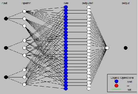
The system model consists of a five-layer ANFIS that takes three inputs (The virtual load of the source cell, the overall state of the target cell and number of users in the entire network). A triangular membership function with 3 linguistic variables was used for each of the inputs. This generates 27 rules that determine the output of each rule. The Model structure is given in fig. 3.

Fig.3 Structure of Proposed ANFIS Model

39 many times larger than the number of parameters being

evaluated [21]. 1500 input/output pairs of training data was used for training. Thus, the ratio between the data points and parameters is about twenty seven times (1500/54).

5.

RESULTS AND CONCLUSION

The ANFIS model was validated using both testing data sets and checking data sets. The testing data sets were presented to the trained ANFIS to see how well the ANFIS model predicts output values. An average testing error of 0.086525 was achieved for an average training error of 0.0067812 using 20 training epochs. The checking data set was used to control the potential of overfitting the data. The checking data and the training data are presented to the ANFIS so that the fuzzy inference model selects parameters associated with the minimum checking data model error. An average checking error of 0.087521 was realized using 1500 input/output checking data set (fig.4).

The ANFIS model uses the hysteresis value for a QoS aware load balancing. The hysteresis increase as the virtual load of the serving eNodeB increases. This increase is gradual before the cell is overloaded (𝜌 ≤ 1𝐶 ). When the serving eNodeB

gets overloaded (𝜌 > 1𝐶 ), the hysteresis value increases

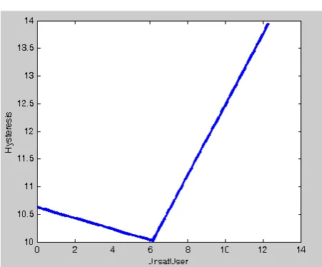
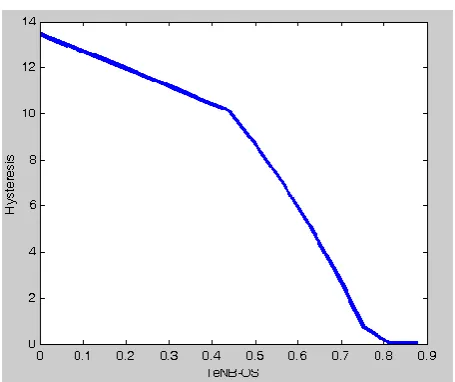
rapidly fig. 5. Before the number of unsatisfied users reaches a certain threshold (in this particular case, 6), the hysteresis tend to decrease with. However, the trend changes spontaneously when the number of unsatisfied users becomes significant (or reaches a certain threshold). The slope of increase in hysteresis when the threshold is attained is much higher than the rate of decrease experienced earlier: see fig.6. The change in hysteresis due to the overall state of the target eNodeB (TeNB-OS) depicts a completely different trend from that of the other two indicators. Generally, the TeNB-OS sets a check on the value of the hysteresis due virtual load and number of unsatisfied users. Between the range 0.0 and 0.45, the decrease in hysteresis due to TeNB-OS is gradual because both the virtual load and number of unsatisfied users contribute to the hysteresis value. The rate of decline in hysteresis becomes more pronounced between TeNB-OS values of 0.45 and 0.75 due to the corresponding negative contribution of the number of unsatisfied users to increasing hysteresis within this range. When the TeNB-OS approaches the value of 1.0, it forces the hysteresis to zero, indicating that the target eNodeB is not able to accept more loads even if the source eNodeB is overloaded, see fig.7.

Fig. 5 Model validation using checking data sets

Fig. 6 Relative contribution of Virtual load to hysteresis value

40

Fig. 8 Relative contribution of target eNodeB overall state users to hysteresis value

In sum, it can be inferred that the virtual load of the source eNodeB plays a more vital load in deciding load balancing. The overall load state of the target eNodeB ensures that the target eNodeB is not overload by the source eNodeB by forcing the hysteresis to zero when it is getting overloaded. The number of unsatisfied users in the entire tends to decrease the load balancing hysteresis when the source eNodeB is not overloaded and increase the hysteresis when the source cell is overloaded because it is a network wide parameter.

6. REFERENCES

[1]StefaniaSesia, IssamToufik and Matthew Baker, “LTE-The UMTS Long Term Evolution: From “LTE-Theory to Practice”, 1st _{edition, John Wiley & Sons, Ltd. , West}

Sussex, UK, 2009.

[2]ETSI TS 136 300, "LTE; Evolved Universal Terrestrial Radio Access (E-UTRA) and Evolved Universal Terrestrial Radio Access Network (E-UTRAN); Overall description; Stage 2" Technical Specification Version 10.4.0 (pg. 176), 2011 Retrieved March., 10, 2012, available at http://www.3gpp.org.

[3]Andreas Lobinger et al, “Load Balancing in Downlink LTE Self-Optimizing Networks”, IEEE 71st VTC 2010, Taipei, Taiwan, June 2010.

[4]Hao Wang et al, “Dynamic Load Balancing in 3GPP LTE Multi-Cell Networks with Heterogenous services”, ICST Conference, Beijing, 2010.

[5]Hao Wang, “Dynamic Load Balancing and Throughput Optimization in 3GPP LTE Networks”, IWCMC 2010, Caen, France, July, 2010.

[6]L. A. Zadeh, “Fuzzy logic, neural networks and soft computing,” in Proc. IEEE Int. Workshop Neuro Fuzzy Control, Muroran, Japan, 1993, p. 1.

[7] G. Chakraborty and B. Chakraborty, “A genetic algorithm approach to solve channel assignment problem in cellular radio networks,” inProc. IEEE Midnight-Sun Workshop Soft Computing Methods in Industrial Applications, Kuusamo, Finland, 1999, pp. 34–39.

[8]B. Dengiz, F. Altiparmak, and A. E. Smith, “Local search genetic algorithm for optimal design of reliable networks,”IEEE Trans. Evol. Comput., vol. 1, pp. 179– 188, June 1997.

[9]X. M. Gao, X. Z. Gao, J. M. A. Tanskanen, and S. J. Ovaska, “Power prediction in mobile communication systems using an optimal neural-network structure,” IEEE Trans. neural Networks, vol. 8, pp. 1446–1455, Nov. 1997.

[10]A.A. Atayero, M.K. Luka, “Applications of Soft Computing in Wireless and Mobile Communications”,

International Journal of Computer

Applications:ISSN0975 – 8887,Submitted.

[11]AmitKonar, "Artificial Intelligence and Soft Computing: Behavioural and Cognitive Modelling of the Human Brain" CRC press, NY, USA, 2000.

[12]R.C.Chakraborty (2010), "Soft Computing Introduction", retrieved on March 18, 2012, available at http:// www.myreaders.info/html/soft_computing.html.

[13]Mathwork Inc., "Fuzzy Logic Toolbox User Guide", Ver., 2.2.14 (2011). Retrieved Jan., 28, 2012 from www.mathworks.com.

[14]Jyh-Shing Roger Jang, "ANFIS: Adaptive Network-Based Fuzzy Inference System", IEEE trans., on Systems, Man and Cybernetics, Vol. 23, No. 3, May-June, 1993, pg. 665-685.

[15]LaureneFausett, "Fundamentals of Neural Networks: Architectures, Algorithms and Applications", 1st edit., Prentice hall, 1993.

[16]MihaiHoriaZaharia, Florin Leon and Dan Gâlea, "Parallel Genetic Algorithms for Cluster Load Balancing", Advances in Intelligent Systems and Technologies Proceedings ECIT2004 - Third European Conference on Intelligent Systems and TechnologiesIasi, Romania, July 21-23, 2004.

[17]William A. Greene, "Dynamic Load-Balancing via a Genetic Algorithm", Proceedings of the 13th International Conference on: Tools with Artificial Intelligence, pg.121-128, 2001.

[18]Ali R. Mehrabian and Morteza M. Zaheri, "Design of a Genetic-Algorithm-Based Steam Temperature Controller in Thermal Power Plants", Advance online publication, engineering Letters, 2007.

[19]Mohammed Jaloun1, Zouhair Guennoun2 and AdnaneElasri, "Use Of Genetic Algorithm In The Optimisation Of The Lte Deployment", International Journal of Wireless & Mobile Networks (IJWMN) Vol. 3, No. 3, June 2011.

[20]Jyh-Shing Roger Jang, "ANFIS: Adaptive Network-Based Fuzzy Inference System", IEEE trans., on Systems, Man and Cybernetics, Vol. 23, No. 3, May-June, 1993, pg. 665-685.

[21]J.-S. Roger Jang and Ned Gulley, "MATLAB Fuzzy Logic toolbox: Computation, Visualization and programming", User Guide vers.1, 1997.

41 Artificial Intelligence (IJARAI):ISSN 2165-4069 Vol.1

No.1, pp.11-16, April 2012.

[23]WINNER, “Assessment of advanced beamforming and MIMO technologies,” WINNER, Tech. Rep. IST-2003-507581, 2005.

[24]ETSI TR 136 942, "LTE; Evolved Universal Terrestrial Radio Access (E-UTRA); Radio Frequency (RF) system scenarios", Technical Report Version 8.2.0 (2009). Retrieved Feb., 20, 2012, from http://www.3gpp.org.

[25]ETSI , Physical layer aspects for E-UTRA Technical Specification Version 8.2.0 . 2006, Retrieved Feb., 20, 2012, from http://www.3gpp.org.

[26]ETSI TS 136 211, "LTE; Evolved Universal Terrestrial Radio Access (E-UTRA); Physical channels and

modulation", Technical Specification Version 10.2.0 ., 2011, Retrieved Feb., 20, 2012, from http://www.3gpp.org.

[27]R. Jain, D.M Chiu and W. Hawe,"A Quantitative Measure of Fairness and Discrimination for Resource Allocation in Shared Systems",Technical Report, Digital Equipment Corporation, DEC-TR-301, 1984.