Plant Biomass, Primary Production and Mineral Cycling of a Mixed Oak Forest in Linnebjer, Sweden

http://dx.doi.org/10.4236/ojf.2014.45061

Plant Biomass, Primary Production and

Mineral Cycling of a Mixed Oak Forest in

Linnebjer, Sweden

Folke O. Andersson

Department of Ecology, Swedish University of Agricultural Sciences, Uppsala, Sweden Email: folke.andersson@slu.se

Received 3 August 2014; revised 17 September 2014; accepted 6 October 2014

Copyright © 2014 by author and Scientific Research Publishing Inc.

This work is licensed under the Creative Commons Attribution International License (CC BY). http://creativecommons.org/licenses/by/4.0/

Abstract

Plant biomass, primary production and mineral cycling were studied in a mixed deciduous forest (Quercus robur L., Tilia cordata L. and Corylus avellana L.) in southern Sweden. Plant biomass amount above and below ground was 201 and 37 t∙ha−1_{, respectively. Primary production above}

and below ground was an estimated 13.3 and 2.3 t∙ha−1_{, respectively. Carbon was the dominant}

element in the forest ecosystem, comprising 133 t∙ha−1_{. Other major elements were: N > Ca > K >}

Si > Mg > S > Mn > P > Fe and Na (range 1123 to 18 kg∙ha−1_{), followed by some trace elements.}

Yearly litterfall restored 6.0 t∙ha−1 _{organic matter or 2.3 t∙ha}−1 _{carbon. Approximately 45%}

de-composed and returned to the soil during the year. Monitoring of other elements revealed that the ecosystem received inputs through dry and wet deposition, in particular 34.4 kg∙ha−1 _{S and 9.4}

kg∙ha−1 _{of N yearly as throughfall. Determination of yearly biomass increase showed that the oak}

forest ecosystem was still in an aggradation or accumulation phase.

Keywords

Plant Biomass, Primary Production, Litterfall, Deposition, Cycling of C, N, P, K, S

1. Introduction

(1981). However, the studies of the mixed deciduous forest in the reserve also included mineral cycling per-formed in the early 1970s, the results of which were never satisfactorily published. Therefore they are not avail-able in the scientific literature, but are still valid, in demand and are hence presented in this paper.

The results can be applied in monitoring changes in tree biomass and production, as well as cycling of ele-ments over time. It is also important to have information on the distribution of eleele-ments in the stand in order to determine temporal changes in air pollution, especially sulfur and nitrogen deposition.

This paper presents the results obtained to date on mineral cycling in the Linnebjer mixed forest. It includes a summary of biomass and primary production by the tree and field layers as essential background and important functional fractions such as litterfall and deposition, as well as data on their contents of elements. The cycling is discussed using a simple model.

2. The Mixed Forest

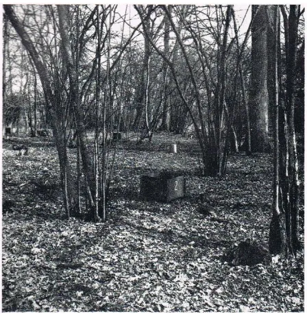
The dominant vegetation in the Linnebjer nature reserve is mixed deciduous forest. Part of the reserve was used as a special area for detailed investigations (Figure 1 andFigure 2). A full description of the vegetation during the study period is given in Andersson (1970b). In brief, the forest has a number of layers: tree layer > 15 m, upper shrub layer 2 - 15 m, lower shrub layer < 2 m and field and bottom layers. The tree layer is dominated by Quercus robur and Tilia cordata and the upper shrub layer by Corylus avellana. The field layer shows seasonal changes, with Anemone nemorosa dominating in spring and Oxalis acetosella in summer. The bottom layer is weakly developed.

3. Element Cycling Model

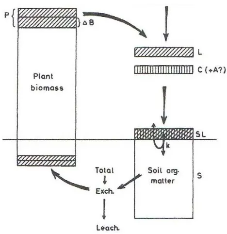
Cycling of elements was assessed using a model developed by Nihlgård (1972) (Figure 3). The analysis was li-mited to the above-ground parts, as root production and the release of nutrients from the root litter and leaching of elements from the soil were not estimated. However, root biomass was measured. In determining the dynam-ics of organic matter in a forest, the above-ground yearly net primary production (P) the yearly litterfall (L) and the decomposition rate (k) are the most important factors. Understanding element cycling requires information on the amounts of elements in the primary plant production, the biomass increase (ΔB), yearly litterfall (L), sur-face litter (SL) and the canopy-leached fraction (CL = the difference between total through fall and incoming rainfall).

Figure 2. Map of the Special area showing ecosystems and sample areas. Key: A. Quercus robur-Oxalis acerosella eco- system; B. Quercus robur-Geumrivale ecosystem; C = Quer- cusrobur-Athyriumfilix-femina ecosystem, D = Clearing phase of ecosystem A and B; E = Filipendula ulmaria ecosystem; F = Carex flacca ecosystem and G = Carex caespitose ecosystem. In the sample area for ecosystem A the situation of 16 litter traps and 12 rain gauges are shown.

4. Methods

4.1. Tree Biomass and Production

A detailed description of the methods developed and applied to the tree layer and the results obtained are pro-vided in Andersson (1970c) and Nihlgård (1972). Therefore, only a summary is given here. The estimates of tree biomass and production were based on allometric regressions, using the relationship between destructive and non-destructive measurements. The estimation procedure comprised four basic steps:

• Stand analyses of non-destructive measurements—tree height and diameter.

• Destructive measurements of sample trees: stem sections or discs, branches, twigs and roots—diameter, age. • Application of the stand data to the regressions of the sample trees obtained in (2).

• Additional observations on e.g. litterfall.

The above-ground biomass and production of trees were studied specifically for 11 Quercus robur, 6 Tilia and Sorbus and 18 Corylus. Studies of the below-ground parts with roots were limited to three individuals of each tree species. The main root biomass fraction, comprising roots > 0.5 cm in diameter, was collected around the tree. The fine root biomass (<0.5 cm diameter) was collected in 10 pits measuring 50 cm × 50 cm × 60 cm excavated along a transect at regular intervals of 2 m.

4.2. Field Layer

The above-ground biomass of the field layer was sampled on occasions corresponding to the maximum devel-opment of the seasonal species. Total primary production was calculated by adding the maximum values ob-tained for the different species investigated. These were sampled in 16 squares (50 cm × 50 cm) selected at ran-dom on each sampling occasion. Below-ground parts were collected within the same squares.

4.3. Litter and Litterfall

Litterfall was collected in 16 litter traps (50 cm × 50 cm × 30 cm) laid out in a systematic way. The trap sides were made of wooden boards and the base of nylon netting and they were placed 20 cm above the ground sur-face. Coarse litter such as twigs and pieces longer than 0.5 m were collected yearly in a 20 cm × 20 cm square sampling area. Random samples of surface litter were taken twice a year, before and after leaf shedding, in 16 squares measuring 50 cm × 50 cm.

4.4. Deposition

In connection with an investigation of element cycling in the oak forest (Andersson 1970b), rain samples were collected and subjected to chemical analysis in order to determine the deposition of sulfur and nitrogen, as well as other incoming nutrients. These samples were collected as through fall in a special area of the forest (Figure 1 and Figure 2).

4.5. Collectors and Collection

The incoming rainfall was measured at a nearby farm 300 m from the throughfall sampling area. A rain gauge of type SMHI with a diameter of 16 cm and fitted with a wind shelter was used (SMHI 1958), placed with the opening 1.5 m above ground. A comparison with data obtained with other gauges used in the forest (see below) showed that the results was usually within the reported range of observations (Nihlgård 1970), although occa-sionally they were 3% lower.

The throughfall was collected in 12 gauges randomly spread in a forested area of 1600 m2. The gauges con-sisted of 1-L polythene bottles with a plastic funnel with diameter 15 cm fitted in the lid. A filter of inert glass wool was placed in the bottom of the funnel to prevent material entering the bottle. To stabilise the gauges, they were placed on the ground inside metal tubes (diameter 16 cm). The top of the gauges was 30 cm above the ground.

4.6. Chemical Analyses of Water

On arrival at the laboratory, the samples were pooled into four composite samples and kept cool (+4˚C). Ana-lyses were carried out within one month as follows:

pH was determined with a pH-meter, type Beckman N-2 (accuracy ±0.02). In calculating average pH, the pH values were first transformed to concentration of hydrogen ions and the average was converted back to pH (cf. Barrett & Brodin 1955).

Further analyses were performed on filtered water. The cations Na, K, Ca, Mg, Fe and Mn were determined on a Perkin-Elmer Atomic Absorption Spectrophotometer, with analytical error normally 1%, estimated from the standard curves.

Chloride concentration was determined with a mercurimetric method using diphenylcarbazon as an indicator

(Clarke, 1950). The accuracy was ±5%, calculated as standard deviation of duplicate analyses (Nihlgård, 1970). Sulphate concentration was determined with a turbidimetric method using BaCl2 and an acid seed solution

(Chesnin Yien, 1950; Rossum & Villarez, 1961). The accuracy ±7%, calculated as for chloride. Phosphate con-centration was determined with a colorimetric method after reduction with ascorbic acid and addition of K-an- timonyltartrate plus ammonium molydate (Murphy & Riley, 1962). The accuracy was ±7%, calculated as above. Nitrate concentration was tentatively determined using a colorimetric method (accuracy ±10%, calculated as above), with alpha-naphthylamine and sulphanilic acid after addition of HAc, BaSO4 and MnSO4 (cfBray, 1945, Method 1, Procedure 1). Ammonia concentration was determined tentatively using Nessler’s regent after addi-tion of sodium potassium tartrate (accuracy ±7%, calculated as above). Total nitrogen concentraaddi-tion was ana-lysed by a macro-Kjeldahl distillation method (Karlgren, 1962). The accuracy was ±6%, calculated as for chlo-ride.

4.7. Soil Sampling and Chemical Analyses

The soil sampling procedure and the methods applied for determination of exchangeable and total amounts of elements are described in full in Andersson, 1970b (pp. 141-146). Statistical analyses are also described in the same publication.

4.8. Statistics

Results are generally presented as means. Percentage errors are given at 95% confidence limit as percentage of the mean. Andersson (1970b) discuss different statistical aspects of errors in sampling and computations.

5. Results

5.1. Biomass and Production of the Tree, Shrub and Field Layers

Biomass and primary production are essential as carrier substances of the elements treated in this paper, so the results presented by Andersson (1970b) for the Linnebjer nature reserve are summarised here. Tree biomass (B) of the mixed forest was estimated to be 238 t∙ha−1, with 201 aboveground and 38 t∙ha−1 belowground (Table 1).

Yearly above-ground primary production (PP) was estimated to be 13.3 t∙ha−1∙yr−1. This included plant losses by death and shedding (L), which amounted to 0.7 t∙ha−1∙yr−1, and plant losses by consumers (G), which amounted to 0.4 t∙ha−1∙yr−1. The below-ground production of tree and understory layers was estimated to be roughly 1.8 t∙ha−1∙yr−1 and fine root biomass production 0.5 t∙ha−1∙yr−1 (Table 1). The above-ground biomass of the field layer was 0.06 - 0.2 t∙ha−1 and its below-ground biomass was 2.4 - 2.6 t∙ha−1 (Table 1and Table 2).

5.2. Element Amounts and Their Distribution in Biomass and in Production Fractions

of the Tree, Shrub and Field Layers

Table 1. Plant biomass and yearly production (t∙ha−1 dry weight at 85˚C) of the tree layer in a mixed woodland with Quercus robur and Corylus avellana. Linnebjer, Sweden.

Biomass Production

Shoot

Overstory trees 155 - 6.3

Quercus robur - 15.8 -

Understory trees 29 2.1

Tilia cordata - 25.5 -

Sorbus aucubaria - 1.6 -

Prunus avium - 0.6 -

Ulmus glabra - 0.6 -

Populus tremula 0.2 -

Shrubs 17 3.0

Corylus avellana -

Field layer 0.2 0.8

Plant losses by death and shedding (L) - 0.7

Plant losses by consumers (G) - 0.4

Total above ground 201 13.3

Root

Main root biomass > 0.5 cm Ø

Quercus robur 27 0.9

Understory trees

Corylus avellana 7 0.9

Fine root biomass < 0.5 cm Ø- 3 0.5

Trees and shrubs

Total below-ground 37 2.3

TOTAL 238 15.6

Table 2. Plant biomass and yearly production (t∙ha−1 dry weight at 85˚C) of the tree layer in a mixed woodland with Quercus robur and Corylus avellana. Linnebjer, Sweden.

Organicmatter C N C/N Na K Ca Mg Mn Fe Si P S

kg∙ha−1 _{ratio g∙ha}−1

Above-ground

Convallaria majalis Oxalis acetosella Other species

Total above-ground kg∙ha−1

10 45 15

70

4.2 18.7

7.3

30.2

0.21 1.73 0.53

2.11

20 14 14

0.419 5.170 2.760

0.008

18.8 126.7

33.4

0.18

119 343 102

0.56

43 148 56

0.25

12 49 12

0.07

1.8 9.4 4.3

0.02

0.8 5.3 2.1

0.01

16.2 96.8 37.7

0.15

16 121

29

0.17 Below-ground

Anemone nemorosa Other species

Total below-ground kg∙ha−1

2320 290

2610

1035 123

1158

49.0 6.5

55.5

21 19

821.4 104.0

0.93

2812 238

3.05

6790 1170

7.96

4400 490

4.89

3820 43

4.25

3320 380

3.70

1550 580

2.13

3366 284

3.65

4990 580

5.57

SUM OF ABOVE-AND

BELOW-GROUND 2680 1188 57.6 0.94 3.23 8.52 5.14 4.32 3.72 2.14 3.80 5.74

Table 3. Mineral content (t∙ha−1 dry weight at 85˚C) of a mixed forest of Quercus robur and Corylus avellana in Linnebjer, Sweden.

Fraction C N C/N Na K Ca Mg Mn P S Fe Si Pb Zn Cu Ni

tha−1 ratio kg ha−1

Above-ground Tree layer Stem wood Stem bark Branches Current twigs Field layer 75.8 8.3 27.1 2.8 0.03 0.219 0.104 0.400 0.081 0.002 346 80 68 35 14 4.8 0.8 4.3 0.6 0.01 148 30 60 30 0.18 200 247 82 30 0.56 25 12 40 10 0.25 12 10 29 9 0.07 9.5 4.2 30.1 5.2 0.15 16.0 9.8 21.6 5.2 0.17 5.8 2.2 5.6 1.5 0.02 30.8 21.7 41.5 16.5 - 0.25 0.12 0.56 0.06 - 0.87 0.20 1.37 0.26 - 0.32 0.09 0.33 0.04 - 0.19 0.07 0.22 0.03 -

Total above-ground 114.0 0.806 - 10.5 268 559 87 60 49.2 52.8 15.1 110.5 0.99 2.70 0.78 0.51

Below-ground

Tree layer Roots > 0.5 cm Roots < 0.5 cm Field layer 15.8 1.6 1.2 0.230 0.031 0.056 69 52 21 5.4 1.1 0.9 8 1 3 142 22 8 17 5 5 6 2 4 12.5 1.5 3.7 20.2 4.3 5.6 16.3 3.8 3.7 111 52.1 - 0.09 0.02 0.09 0.36 0.13 0.33 0.13 0.02 0.03 0.11 0.04 0.03

Total below-ground 18.6 0.317 - 7.4 12 172 27 12 17.7 30.1 23.8 163.1 0.20 0.82 0.18 0.18

TOTAL ABOVE-AND

BELOW-GROUND 132.6 1.123 - 17.9 280 731 114 72 66.9 82.1 38.9 273.6 1.19 3.52 0.96 0.69

Table 4. Comparison of the element distribution in the biomass of a mixed forest of Quercus robur and Corylus avellana in Linnebjer, Sweden, with that in neighboring beech forests along a fertility gradient in southernmost province in Sweden.

Forest type Base

saturation %

Basal

area m2_∙ha−1 _t∙haC −1

N P Na K Ca Mg Mn Fe S

kg∙ha−1

Oak Oxalis Beech Mercurialis

Lamium Deschampsia 21 60 22 12 31 31 31 30 114 156 159 119 81 83 106 64 49 55 85 65 11 24 32 17 268 465 460 318 559 924 663 478 87 121 105 85 60 2 111 29 15 6 15 5 53 59 68 65

From: Oak (Andersson, 1970b); Beech (Nihlgård & Lindgren 1977).

lity in the form of exchangeable amounts in soil and in total biomass. Other elements such as P, Mn and Fe are dependent on the degree of solubility, which is regulated by soil pH. Sulfur to some extent reflects atmospheric deposition.

5.3. Amounts of Elements in Litterfall and Surface Litter

In order to analyse the circulation of elements, data on yearly litterfall (L) and the dynamics of the surface litter (SL) were used (Table 5).

The nitrogen content in the annual litterfall was 69 kg∙ha−1. The other elements were present in the following descending order: Ca, Si, Mg, K, S, Mn, P, Fe and Na, in amounts ranging from 41 to 0.9 kg∙ha−1∙yr−1. The sur-face litter comprised 6.0 t∙ha−1 organic matter, or 2.8 t∙ha−1 of carbon with a nitrogen content of 107 kg∙ha−1. The other elements occurred in the following descending order: Ca, Si, S, Mg, Mn, K, P, Fe and Na, in amounts ranging from 59 to 0.8 kg∙ha−1.

Some readily mobile elements, such as K and Na, had a decomposition rate (k-value) of approx. 50%, indi-cating that half the litterfall amount was turned over during one year. Other elements such as Si had a slow turnover rate of 14%, while the rest had intermediate values.

5.4. Amount of Elements in Precipitation, Throughfall and Interception

Input of elements was the result of precipitation measured in the open field (In), and of not measured dry depo-sited, aerosols (A) (Table 6 and see Figure 1).

Content of elements (kg∙ha−1) in incoming precipitation (In), throughfall (T) and interception (Diff = canopy − leached fraction) in a mixed forest of Quercus robur and Corylus avellana in Linnebjer, Sweden (Table 6).

Table 5. Content of organic matter and elements in litterfall (L) and surface litter (SL) and decomposition factor k (L/L + SL) of a mixed forest of Quercus robur and Corylus avellana in Linnebjer, Sweden, April 1966-March 1967.

Period Fraction Org.

matter C N Na K Ca Mg Mn Fe Si P S

kg∙ha−1 April 66- June 66 Twigs Leaves Budscales Misc. 245 53 310 8 120 26 152 4 3.72 1.71 6.17 0.08 0.06 0.01 0.04 0 0.34 0.15 0.52 0.02 1.88 0.43 2.79 0.04 0.27 0.12 0.60 0.02 0.18 0.04 0.26 0.01 0.04 0.01 0.07 0 0.45 0.16 0.70 0.02 0.16 0.06 0.36 0.01 0.23 0.07 0.27 0.02 July 66- Sept. 66 Twigs Leaves Budscales Misc. 238 212 204 174 117 104 100 85 2.52 4.37 4.06 4.11 0.06 0.08 0.03 0.05 0.34 0.82 0.79 0.31 2.06 1.90 1.83 1.81 0.20 0.44 0.39 0.33 0.14 0.29 0.17 0.16 0.09 0.04 0.05 0.05 0.57 0.58 0.48 1.70 0.13 0.24 0.24 0.27 0.22 0.27 0.18 0.16 Oct. 66- Nov. 66 Twigs Leaves Budscales Misc. 87 1491 110 49 43 151 54 24 0.85 17.59 2.19 1.01 0.02 0.10 0.02 0.02 0.13 2.27 0.19 0.15 0.65 13.69 0.99 0.46 0.08 2.32 0.21 0.12 0.06 2.13 0.09 0.05 0.03 0.32 0.03 0.21 0.17 6.26 0.26 0.59 0.04 0.79 0.13 0.08 0.07 1.43 0.10 0.10 Dec. 66- March 67 Twigs Leaves Budscales Misc. 465 1048 0 38 228 514 - 19 5.07 14.29 - 0.87 0.09 0.27 - 0.01 0.46 0.66 - 0.05 3.15 9.46 - 0.28 0.29 0.74 - 0.03 0.20 0.58 - 0.02 0.14 0.58 - 0.06 2.41 6.37 - 0.56 0.21 0.61 - 0.05 0.56 1.65 - 0.09 Total Twigs Leaves Budscales Misc. 1035 2840 624 269 508 1375 306 172 12.16 38.66 12.42 6.07 0.23 0.46 0.09 0.08 1.27 3.90 1.50 0.53 7.74 25.48 5.61 2.59 0.84 3.62 1.20 170 0.58 3.04 0.52 0.24 0.30 0.95 0.15 0.32 3.60 13.37 1.47 2.87 0.54 1.70 0.73 0.41 1.08 3.42 0.55 0.37

Total litterfall (L) 4768 2321 69.31 0.86 7.20 41.42 7.36 4.38 1.72 2.31 3.38 5.42

Surface litter (SL) Finer fractions Branches 6010 4400 1670 2825 1985 840 107 99 7.8 0.75 0.60 0.15 6.63 5.00 1.63 58.92 44.92 14.00 8.65 7.39 1.29 7.30 6.29 1.01 3.43 2.77 0.66 128.07 118.20 9.87 4.47 3.87 0.60 13.86 12.07 1.79 TOTAL LITTER

(L + SL) 10,778 5146 176.3 1.61 13.83 100.34 16.04 11.68 5.15 149.38 7.85 19.28

k-value 0.44 0.45 0.39 0.53 0.52 0.41 0.46 0.38 0.20 0.14 0.43 0.28

or absorbed elements (negative values) in the canopy. The Diff value also included possible dry deposited aero-sols (A). What were possibly overlooked were elements from A that had been absorbed into the leaves. This can be the case e.g. for NO3 and NH4ions.

The amount of precipitation in the year of measurement (1967) was 644 mm. The amount captured by the canopy, interception, was 168 mm. The input of elements with rain was in decreasing order: Cl, S, N, Na, Ca, Mg, K, Mn and P in amounts ranging from 23 to 0.04 kg∙ha−1∙yr−1. The through fall contained in decreasing or-der: Cl, K, S, N, Na, Ca, Mg, Mn and P, in amounts ranging from 55 to 1.5 kg∙ha−1∙yr−1. The higher values show the most readily motile elements.

Special consideration needs to be given to deposition of sulfur and nitrogen. The open field received inputs of 11.0 kg S ha−1∙yr−1 and 9.4 kg N ha−1∙yr−1. The through fall contained 34.3 S and 22.3 N kg∙ha−1∙yr−1. Over time, these amounts would contribute to acidification of the soil and one-sided fertilisation of the forest. The study area was located in a rural landscape not far from urban areas, which may explain the very high level of S, but also the unexpectedly high level of N. The levels observed were lower than those reported for the north-west of the region at the time (Nihlgård 1972). Since then, S deposition has strongly decreased and the Slevel in the open field today is approx. 5 kg∙ha−1∙yr−1. The present day N deposition rate is approximately 10 kg∙ha−1∙yr−1

(Pihl-Karlsson et al. 2012).

5.5. Soil Organic Matter and Exchangeable Mineral Content

Table 6. Content of elements (kg∙ha−1) in incoming precipitation (In), throughfall (T) and interception (Diff = canopy-

leached fraction) in a mixed forest of Quercus robur and Corulys avellana in Linnebjer, Sweden.

Period Precipitation Na K Ca Mg Mn Cl S P Ntot pH

type mm kg∙ha−1

2-24/12 1966 In T Diff 81.5 68.2 −13.3 2.23 7.95 +5.72 0.19 1.92 +1.73 0.83 2.92 +2.09 0.29 1.04 +0.75 0.02 0.21 +0.19 3.88 12.58 +8.70 1.60 4.74 +3.14 0.006 0.015 +0.009 0.97 1.17 +0.20 5.2 4.8 25/12 1966- 24/1 1967 In T Diff 65.5 55.1 −10.4 1.79 2.71 +0.92 0.08 1.25 +1.17 0.42 1.40 +0.98 0.25 0.58 +0.33 0 0.14 +0.14 4.00 4.51 +0.51 1.11 3.26 +2.15 - - - 1.14 1.10 −0.04 4.9 4.7 25/1-21/2 1967 In T Diff 32.0 25.1 −6.9 0.54 nd nd 0.04 2.19 +2.15 0.31 1.81 +1.50 0.10 0.65 +0.55 0 0.16 +0.16 1.27 8.59 +7.32 0.10 3.77 +3.67 0.001 0.003 +0.002 1.16 2.67 +1.51 4.4 6.2 22/2-6/3 1967 In T Diff 5.0 4.9 −0.1 0.02 0.38 +0.36 0 0.16 +0.16 0.05 0.27 0.22 0.01 0.11 +0.10 0 0.03 +0.03 0.16 0.69 +0.53 0.03 0.82 +0.79 0 0 0 0.01 0.04 +0.03 4.7 4.7 7-24/3 1967 In T Diff 31.5 29.1 −2.4 0.23 0.43 +0.20 0.04 0.62 +0.58 0.35 1.11 +0.76 1.63 5.16 +3.53 0 0.13 +0.13 2.42 4.33 +1.91 0.99 2.65 +1.66 0.001 0.002 +0.001 0.04 0.15 +0.11 4.6 4.7 25/3-6/5 1967 In T Diff 37.0 27.1 −9.9 0.90 1.06 +0.26 0.06 0.54 +0.48 0.30 1.17 +0.87 1.57 2.49 +0.92 0 0.10 +0.10 2.51 2.16 −0.35 0.93 2.19 +1.26 0.001 0.011 +0.010 1.64 3.06 +1.42 5.0 5.9 7-19/5 1967 In T Diff 42.0 32.5 −9.5 0.14 0.73 +0.59 0.13 0.56 +0.43 0.26 0.70 +0.44 0.05 0.23 +0.18 0.01 0.12 +0.11 0.50 2.01 +1.51 0.56 1.56 +1.00 0.001 0.004 +0.003 0.49 0.98 +0.49 5.5 5.4 20/5-19/6 1967 In T 37.5 27.6 0.13 0.78 0.14 12.35 0.30 1.08 0.09 0.90 0.04 0.30 1.17 2.47 0.88 2.07 0.012 1.158 0.69 3.65 5,1 6,1

Diff −9.9 +0.65 +12.21 +0.78 +0.81 +0.26 +1.30 +1.19 +1.146 +2.96

20-30/6 1967 In T Diff 48.5 34.3 −14.2 0.14 0.86 +0.72 0.05 2.35 +2.30 0.36 0.79 +0.43 0.05 0.35 +0.30 0.02 0.12 +0.10 0.48 2.06 +1.58 0.53 1.60 +1.07 0.003 0.051 +0.048 0.07 0.93 +0.86 5.5 5.8 1-16/7 1967 In T Diff 74.5 49.8 −24.7 0.15 0.94 +0.79 0.07 2.32 +2.25 0.68 0.84 +0.16 0.07 0.34 +0.27 0.16 0.16 0 1.09 2.78 +1.69 1.09 2.13 +1.04 0.002 0.031 +0.029 0.64 2.95 +2.31 5.0 5.0 17/7-18/8 1967 In T Diff 42.0 34.3 −7.7 0.22 0.67 +0.45 0.17 2.58 +2.41 0.34 0.76 +0.42 0.07 0.29 +0.22 0.01 0.11 +0.10 2.01 2.73 +0.72 0.29 1.09 +0.80 0.002 0.078 +0.076 0.24 1.88 +1.64 5.6 6.1 19/8-29/9 1967 In T Diff 38.0 20.6 −17.4 0.25 0.49 +0.23 0.10 2.91 +2.81 0.30 0.68 +0.38 0.08 0.26 +0.18 0.04 0.13 +0.09 1.58 3.51 +1.93 0.67 1.57 +0.90 0.003 0.119 +0.116 0.60 1.74 +1.14 5.8 6.8 30/9-13/10 1967 In1 T Diff 61.5 43.8 −18.7 0.42 1.08 +0.66 0.14 5.02 +4.88 0.49 1.40 +0.91 0.13 1.04 +0.91 0.03 0.24 +0.21 0.71 2.39 +1.68 1.18 4.12 +2.94 0.004 0.066 +0.062 0.95 1.28 +0.33 nd 5.9 14/10-1/11 1967 In T Diff 20.5 10.4 −10.1 0.43 0.35 −0.08 0.05 1.11 +1.06 0.16 0.71 0.55 0.05 0.41 +0.36 0.01 0.19 +0.18 0.03 2.47 +2.44 0.53 1.55 +1.02 0.001 0.002 +0.001 0.47 0.32 −0.15 5.1 6.2 2-21/11 1967 In T Diff 26.5 14.9 −11.6 0.11 0.27 +0.16 0.03 1.50 +1.47 0.18 0.64 +0.46 0.32 0.27 −0.05 0.02 0.13 +0.11 0.21 1.37 +1.16 0.50 1.28 +0.78 0.002 0.003 +0.001 0.33 0.42 +0.09 5.1 5.7 TOTAL In T Diff 643.5 476.7 −166.8 7.71 18.70 +10.99 1.29 37.38 +36.09 5.33 16.28 +10.95 4.76 13.83 +9.07 0.36 2.27 +1.91 23.02 54.65 +31.63 10.99 34.43 +23.44 0.039 1.543 +1.504 9.44 22.34 +12.90 − −

6. Discussion

Element cycling is currently a central theme in ecosystem ecology (Ågren & Andersson 2012, Andersson 1970a). The main results of the present study are summarised in Table 8. The yearly biomass increase indicates that at the time of measurement, the Linnebjer forest ecosystem is still in an aggradation or accumulation phase

(Bormann & Likens 1979). Tree biomass increased yearly by 6.6 t∙ha−1 or 3.1 t∙ha−1 carbon. The other elements accumulated in the order: N > Ca > Mg > K > Mn > Si > P, in amounts ranging from 29 to 1.8 kg∙ha−1 yearly. The litterfall returned elements to the soil. 14% - 53% was decomposed and returned to the ecosystem over the year. It can thus be assumed that the exchangeable pool of elements was slightly increasing. The atmospheric deposition of sulfur observed was sufficient to cause acidification of the forest soil. The nitrogen input should have had a fertilising effect, leading to increased forest growth.

The results reported deal with plant biomass, primary production and mineral cycling. Earlier the two first properties have been reported, but the mineral cycling not. As the results still are valid and can serve as refer-ence material, it is considered essential to have them published. The cycling of carbon, nitrogen and sulfur are elements, which are affected by a changing climate and deposition. Repeated investigations make it possible to address questions like the forest as a source or sink forcarbon.

The result of plant biomass and production are less affected by time as the methods are considered as more or less the same today. Chemical methods and techniques have changed more. The results related to chemistry and reported are, however, considered as “robust” and will allow being used for comparisons. Even if “modern” chemical methods are used, the final results are depending on the quality of the data from the estimation of plant biomass and production.

In a follow up paper, results from an investigation of sampling in vegetation and soil after fifty years will be reported.

Acknowledgements

These investigations were carried out at the former Department of Ecology, University of Lund, under the lea-dership of Professor Nils Malmer. The work took place over a long period leading to a PhD degree in 1970. Mineral cycling of the oak forest was intended to be a part of the PhD thesis, but the analysis had to be post-poned for practical reasons. A number of people assisted in the work. Laboratory assistance was provided by, among others, Anita Balogh, Maj-Lis Gernersson and Mimmi Varga. Field assistance was provided by a ne-

Table 7. Distribution of elements in soil organic matter (SOM) and amount in an extraction with ammonium acetate (Am- Ac.Exch) in the soil profile of a mixed forest of Quercus robur and Corylus avellana in Linnebjer, Sweden.

Fraction Organic matter C N C/N Na K Ca Mg Mn P

t∙ha−1 _{ratio kg∙ha}−1

Soil organic matter 0 - 60 cm Am-Ac. Exch 0 - 40 cm

288 -

108 -

12.0 -

9 -

- 221

- 226

- 532

- 242

- 55

- 256

Table 8. Distribution of organic matter and chemical elements in some important above-ground functional fractions and turnover characteristics of a mixed forest of Quercus robur and Corylus avellana in Linnebjer, Sweden.

Symbol Fraction Biomass C N C/N Na K Ca Mg Fe Mn P Si

t∙ha−1 _{ratio kg∙ha}−1

PP ΔB L CL

R SL SOM Exch

Yearly primary production Yearly biomass increase Yearly litterfall Canopy leached fraction Input by rain

Surface litter Soil organic matter Exch. in soil PP-ΔB L + CL L/L + SL

12.8 6.6 4.8 - - 6.1 288 - 6.2

- 0.44

6.33 3.06 2.32 - - 2.83 108 - 3.27

- 0.45

0.165 0.029 0.070 0.013 0.009 0.110 12

- 0.136

0.11 0.39

38 106

33 - - 26

9 - - - -

1.17 0.26 0.86 10.99

7.71 0.75 - 221 0.91 11.74

0.53 49.4

8.9 7.2 36.1

1.3 6.6 - 226 40.4 43.3 0.52

66.8 20.3 41.4 11.0 5.3 58.9

- 532 46.5 54.4 0.41

24.1 14.0 7.4 9.1 4.8 8.7 - 242 10.8 16.4 0.46

1.51 0.42 1.72 - - 3.43

- - 1.09

- 0.33

13.6 8.3 4.4 1.4 0.4 7.3 - 55 5.3 6.3 0.38

9.6 1.8 3.8 1.5 <0.1

4.5 - 421

7.5 5.3 0.46

27.3 2.8 21.3

- - 128

- - 24.6

ver-failing study mate, Jan Ericsson, and staff at the Botanical Garden, Lund. Many measurements and sam-plings were performed by a local farmer.

The scientific work involved intense collaboration and exchanges over the years with Professor emeritus Bengt Nihlgård, Lund, who shared the final work. Scientifically, I am also indebted to Professor emeritus Göran Ågren, Uppsala, whose collaboration was an essential factor in finalising this work.

The Swedish Natural Science Research Council provided the main funding for the research.

References

Ågren, G. I., & Andersson, F. O. (2012). Terrestrial Ecosystem Science—Principles and Applications (pp. 230). Cambridge: Cambridge University Press.

Andersson, F. (1970a). An Ecosystem Approach to Vegetation, Environment and Organic Matter of a Mixed Woodland and Meadow Area. Thesis, Lund.

Andersson, F. (1970b). Ecological Studies in a Scanian Woodland and Meadow Area, Southern Sweden. I. Vegetational and Environmental Structure. Opera Botanica, 27, 190.

Andersson, F. (1970c). Ecological Studies in a Scanian Woodland and Meadow Area, Southern Sweden. II Plant Biomass, Primary Production and Turnover of Organic Matter. Botaniska Notiser, 123, 8-51.

Barrett, R. H., & Brodin, G. (1955). The Acidity of Scandinavian Precipitation. Tellus, 7, 251-257.

http://dx.doi.org/10.1111/j.2153-3490.1955.tb01159.x

Bormann, F. H., & Likens, G. E. (1979). Pattern and Processes in a Forested Ecosystem (pp. 253). New York: Springer Verlag. http://dx.doi.org/10.1007/978-1-4612-6232-9

Bray, R. H. (1945). Nitrate Tests for Soil and Plant Tissues. Soil Science, 60, 219-221.

http://dx.doi.org/10.1097/00010694-194509000-00003

Chesnin, L., & Yien, C. H. (1950). Turbidimetric Determination of Available Sulphates. Soil Science Society of America Journal, 15, 149-151. http://dx.doi.org/10.2136/sssaj1951.036159950015000C0032x

Clarke, F. E. (1950). Determination of Chloride in Water. Analytical Chemistry, 22, 553-555.

http://dx.doi.org/10.1021/ac60040a011

Karlgren, L. (1962). Vattenkemiska Analysmetoder. Limn. Inst. Uppsala. Mimeographed, 115.

Murphy, J., & Riley, J. P. (1962). A Modified Single Solution Method for Determination of Phosphates in Natural Waters. Analytica Chimica Acta, 27, 31-35. http://dx.doi.org/10.1016/S0003-2670(00)88444-5

Nihlgård, B. (1970). Precipitation, Its Chemical Composition and Effect on Soil Water in a Beech and a Spruce Forest in South Sweden. Oikos, 21, 208-217. http://dx.doi.org/10.2307/3543676

Nihlgård, B. (1972). Plant Biomass, Primary Production and Distribution of Chemical Elements in a Beech and a Planted Spruce Forest in South Sweden. Oikos, 23, 68-91. http://dx.doi.org/10.2307/3543928

Nihlgård, B., & Lindgren, L. (1977). Plant Biomass, Primary Production and Bioelements of Three Mature Beech Forests in South Sweden. Oikos, 28, 95-104. http://dx.doi.org/10.2307/3543328

Pihl-Karlsson, G., Akselsson, G., Hellsten, S., Kronnäs, V., & Karlsson, P. E. (2012). The State of the Forest Environment in Scania. Report B 205, Gothenburg: The Swedish Environment Institute, IVL, 33 p. (In Swedish)

Reichle, D. E. (1981). Dynamic Properties of Forest Ecosystems. International Biological Programme 23. Cambridge: Cambridge University Press.

Rossum, J. R., & Villarez, P. A. (1961). Suggested Method for Turbidimetric Determination of Sulfate in Water. American Water Work Association, 53, 873-876.