Graph Rigidity Application for Localization in WSN
Shamantha.Rai.B
IIIT-Allahabad
Shirshu. Varma
Phd,IIIT-Allahabad
ABSTRACT
Localization in WSN involves the global discovery of node coordinates. In a network topology, a few nodes are deployed to known nodal locations and remaining node nodal location information are dynamically estimated using with algorithms. The nodes of sensor network are of random type and the topology of network varied dynamically, as a result the most of the localization techniques fails in locating exact positions. The different solution’s that are already available succumbs to measure noise. We propose an algorithmic approach using the concept of graph rigidity, where a sensor graph is drawn to make use of network topology to form globally rigid sub-graphs.
Keywords
WSN Localization,Rigid graphs, coordinate transformations, trilateration.
1. INTRODUCTION
Wireless sensor networks (WSNs) are high-flying part of research in the modern epoch. The WSNs are cheap, battery operated, can achieve multiple functions, and hence they are appropriate for broad range of applications varying from health monitoring, animal tracking, road traffic monitoring, intrusion detection, environment monitoring, habitat monitoring, military and surveillance etc. WSN nodes must be able to self -localize, this is the most desirable characteristic that ought to be inculcated in the WSN nodes, consecutively to prop up the variety of applications. For all applications, the gathered data will be not prolific if we are incapable to get the precise positions of the WSN nodes. There are also drastically changes in the routing techniques for WSNs. Recently, location aided geographic routing is gaining prominence due to its uncomplicated and well-organized design. Such location aided routing also requires exact positions of the WSN nodes to for effective and efficient data exchange among nodes and base station. The location information is utilized to steer routing path discovery and packet forwarding, thus facilitating the best route, reducing energy utilization and optimizing the network. In routing based on location and its services, finding out relative locations of the WSN nodes with minimal estimation error is quite important. Hence, in past few years to bring-up the aforesaid applications, a range of localization techniques as described in [20], [21], [2], [3], and [13] were designed and implemented thoroughly. These techniques have a varying amount of estimation error and some among these techniques are not apposite, in favour of all the applications. Accordingly, there is prerequisite of a proficient localization technique. The concept of graph rigidity is thoroughly explained in [8], [9], [12], [16] and [17]. Research is carried on in localization using the concept of graph rigidity. Rigid graphs are more efficient than the prior graph theory related distance measurement localization techniques because their distances remain intact with homogeneous coordinate transformations. The sensor network localization algorithms are mainly based the following criteria as mentioned in [10]:
Sensitivity to noise in the measured distance
Sparse connectivity
Scalability to large networks
Centralized/Distributed algorithms
It is to be noted that distributed algorithm is much harder than the centralized algorithm; actually distributed approach can be applied to the centralized approach, but vice versa is not feasible. Centralized algorithms are better suited for providing accurate location estimates than the distributed algorithms. But the centralized algorithms suffer from scalability problem, the algorithm fails when implemented for a large scale sensor networks. The other main disadvantage in centralized algorithm is that, it has multi hop transmission over the network, leading to information loss or inaccurate information. The computational complexity is extremely high. Computation is done in a single base station which might go ahead with single point of failure. Distributed algorithms such as in [11] are further more complex to design because there is an obscured relationship between local behaviour and global behaviour i.e. algorithms might be optimal in the local maps but might not be optimal in the global maps. Error propagation is also another setback in distributed approach. Distributed approach will have multiple iterations to resolve the problem which will seize long time for localization than acceptable. Most of the algorithms in literature are distributed, but suffer from the noisy inter sensor data and do not scale to the expandable size of the network. The previous graph related algorithms [19] and [14] were providing mere connectivity between the nodes and there was localization error.
2. RELATED WORK
Savvides et al in [7] have developed Ad-hoc positioning (APS) where we have certain nodes as landmarks to which range estimation is done using hop counts (DV-hop) or distance measurements (DV-distance). In APS hop counts are calculated between any given two landmarks and then average distance per hop is estimated. Then multilateration is used to find the locations.
Eren et al. in [4] provides a theoretical base for network localization using the provision of graph rigidity theory. Authors argue that WSN is uniquely localizable if and only if its obtained sub- graph is generically globally rigid (GGR). In addition, they have revealed that definite subclass of globally rigid graphs called as trilateration graphs can be made and localized in linear time. Adding more too global rigidity and trilateration graphs they have built robust quadrilaterals. These robust quadrilaterals tend to offer localizations without any ambiguity and bear the measurement noise.
estimate its distance to neighbours and here absolute position references like GPS or anchor nodes are not given. Since it is implemented in physical network accuracy and performance of algorithm is easily calculated. This is a distributed localization algorithm that localizes nodes in areas constructed by robust quadrilaterals. The distributed algorithm is designed for localizing nodes in a WSN where nodes have capability of approximating distance to neighbouring WSN nodes but such measurements are ruined by noise. The graph realization over here is hard for reasons that:
There is deficient data due to which computation of a unique position assignment for every node is difficult. Noisy distance measurements
No absolute reference point or anchor nodes that form a great starting point for localization.
Designing an algorithm that can scale linearly with network size is hard.
The flip ambiguities can be evaded by using the robust quads which could otherwise lead to in correct localization computations. The robust quads could manage a certain amount of measurement noise. But this algorithm will fail if node connectivity is less and high measurement noise is high. In brief the localization algorithm works as follows: Every WSN node measures its distances to neighbouring nodes and relays this measurements. This “one-hop” information is adequate for every node to localize itself and its neighbours which is termed as a cluster in local coordinate system. Then a coordinate transformation between the overlapping clusters is computed. Many cluster based methods were designed, but failed due to the localization errors caused by flip ambiguity.
Aspnes et al in [5] provides a theoretical groundwork for solving the WSN localization problem. Here too he has considered some nodes in which in prior have their location information and the remaining nodes have to find out its locations by assessing the distances to the immediate neighbours. Modelling of WSN localization is done by using the notion of grounded graphs. Graph rigidity theory is used to investigate clauses for unique localizability. They have further studied the computational complexity of WSN localization.
Koren et al in [3] describes an algorithm for WSN localization using the small inter-sensor distances. The algorithm is totally decentralized. It splits the graph into “patches” and computes local coordinates. All the patches are fixed together by making use of distributed global optimization process. This technique is highly robust even if there is existence of noisy measurements than incremental methods which are available. Contrasting with some other global optimization techniques this technique cannot be duped by local minima. The local minima usually lead to foldovers in the network arrangement. The algorithm is anchor free, and hence prior information about locations of some sensors is not needed. However there is a procedure available to make the most of identified locations of any number of anchors. In noisy environments where the sensors are distributed over regions with a variety of geometric shapes.
Anderson et al in [10] states that graph theory has been employed to portray solvability of the wireless sensor network localization problem. The WSN nodes are represented as vertices and edges correspond to sensor node pairs among which the distance is known. In range based sensor network localization an important outcome is that if the sub graphs of the sensor network graph is generically globally rigid, and there is a right set of anchors at needed positions, then the
network can be localized. For planar graph problems if the sensor network graph is given with three or more non collinear anchor nodes at specified points then all the WSN nodes will be situated at generic points. The inter sensor distances analogous to the graph edges are accurately known without being affected by evaluated noise. For WSN to be localizable GGR of a graph is the necessary. In practical approach distance measurements by no means will be correct. The equations can never find solutions which will produce exact sensor node positions. This paper argues that if the error in distance measurement is not too high and the related graph is generically globally rigid including some non collinear anchor nodes, then the sensor network graph will be fairly accurately localizable.
Goldenberg et al in [15] have designed a complete framework for localization with an efficient component which correctly verifies which WSN nodes are localizable and which WSN nodes cannot be localized. Implementing this system, they have accomplished broad assessment of network localizability because it affects network design and deployment. The method for identifying localizable WSN nodes is robust even if there are edge length errors to be practical. Routing in partially localizable networks is also dealt with integration of geographic routing with location information of WSN nodes and geographic routing without location information of WSN nodes. Evaluation and shows that such novel cross layer integrations improves network performance. In [19] they argue that the localization algorithms in literature algorithms do not provide guarantee on correctness of methodology. They even expect the network density to be larger than actually needed for unique localizability. Here authors have described sweeps. Sweeps considers bilateration networks and localizes them accurately. In Sweeps algorithms angle measurements and noisy distance measurements are taken care efficiently. Extensive simulations have shown that sweeps localizes networks containing thousands of nodes in fewer minutes. Sweeps works out best for sparse networks. Sweeps are incremental approach based and hence it will be implemented in distributed manner. Sweeps can also be extended for optimized coverage controlled mobility, spatial coverage and optimized localizability.
3. DEFINITIONS and THEOREMS
3.1.1 Basic Definitions
A configuration is a finite collection of n labeled points,
𝑝 = (𝑝1, … . . , 𝑝𝑛), where 𝑝𝑖
∈
𝐸𝑑, for1 ≤ 𝑖 ≤ 𝑛.A bar framework in 𝐸𝑑 is a graph G with n vertices together
with a corresponding configuration 𝑝 = (𝑝1, … . . , 𝑝𝑛) in 𝐸𝑑 and is denoted by 𝐺(𝑝).
Two frameworks 𝐺(𝑝) and 𝐺(𝑞) are equivalent, i.e. 𝐺(𝑝) =
𝐺(𝑞), if when {𝑖, 𝑗} forms an edge of G, then |𝑝𝑖− 𝑝𝑗| =
|𝑞𝑖− 𝑞𝑗|
Configuration 𝑝 = (𝑝1, … , 𝑝𝑛) is congruent to 𝑞 =
(𝑞1, … . , 𝑞𝑛), and we write 𝑝 = 𝑞 , if for {𝑖, 𝑗} in
{1, … , 𝑛}, |𝑝𝑖− 𝑝𝑗| = |𝑞𝑖− 𝑞𝑗|.
A framework G(p) is called globally rigid in 𝐸𝑑if 𝐺(𝑝) =
A configuration𝑝 = (𝑝1, … , 𝑝𝑛) in 𝐸𝑑 is such that its coordinates are algebraically independent, we say p is generic.
For a given graph 𝐺, when 𝐺(𝑝) is globally rigid for all generic configurations 𝑝 in 𝐸𝑑 we say that 𝐺 is generically globally rigid (GGR).
A framework is called flexible if we have a continuous deformation starting from the known configuration to another, such that edge lengths are preserved. If no such deformation exists, then it is called rigid.
A rigid framework is minimally rigid if it becomes flexible after an edge is removed.
A rigid framework is redundantly rigid, if it remains rigid upon the removal of any edge.
K-connectivity: A graph is defined as k-vertex connected if it is connected even after removing k-1 vertices. Otherwise a graph is k-vertex connected if all pair of vertices is connected by no less than k disjoint paths.
While considering a planar graph the essential condition for a graph to be GGR is 3- connected. This means the graph should remain connected even after removing two of its vertices. 3-vertex connectivity can be generalised as a graph whose minimum in-degree is 3.
3.1.2 Theorems
The following theorems deal with the GGR of a graph. 1. Laman Theorem: According to [17], A graph is
generically, minimally rigid in 2D if and only if it has 2𝑛 − 3 edges and no sub-graph of k vertices has more than 2𝑘 − 3 edges.
2. Consider a graph 𝐺(𝑉, 𝐸) with number of vertices n such that ≥ 4 , and graph is GGR if and only if it is 3-connected and redundantly rigid. In 𝑅3 the graph is GGR if and only if it is 4-connected and generically redundantly rigid.
4. METHODOLOGY
The implementation of the DLGR algorithm is divided into three different tasks which are described separately:
4.1 Network Deployment
While deploying a sensor network following assumptions are considered:
4.1.1 A sensornet having n number of WSN nodes in a specified area
In 2-D coordinate plane “n” number of WSN nodes is deployed randomly within a certain boundary area. The value “n” varies from hundreds to hundreds of thousands.
4.1.2 Connectivity based on transmission range
A specific transmission range is specified for each sensor node of the sensornet, which is capable of communicating with other WSN nodes inside this transmission range. Each sensor node will also be given with a unique id to resolve any ambiguity if occurred.
4.1.3 Finding neighbors of WSN nodes in a sensornet who are within range requirements
In 2-D coordinate system the inter sensor distances between any two WSN nodes is calculated using the distance formula. If (𝑥1, 𝑦1) and (𝑥2, 𝑦2) are the coordinates of two sensors then the distance D is:
𝐷 = 𝑥 2− 𝑥1 2
+ 𝑦2− 𝑦1 2
A sensor is a neighbour of other if and only if 𝐷 ≤ 𝑅, where R is the transmisson range
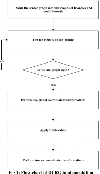
4.2 Distributed Localization using Rigid Graphs(DLRG) We design a new a new algorithm for sensor network localization which is distributed and which uses the concept of rigid graphs (as defined in 3). The flow chart of the DLRG is shown in figure 1.
Divide the sensor graph into sub-graphs of triangles and quadrilaterals
Test for rigidity of sub-graphs
Is the sub-graph rigid?
Perform the global coordinate transformations
YES
Apply trilateration
Perform inverse coordinate transformations
[image:3.595.324.521.250.593.2]NO
Fig 1: Flow chart of DLRG implementation
The DLRG algorithm is divided into following two phases:
4.2.1 Sub-graphs generation from the sensornet We start with a vertex V(i) and find the immediate 1-hop neighbours, whose distance 𝑑𝑖𝑗 is known, continuing in the identical manner we uncover the globally rigid triangles and quadrilaterals which satisfy the theorem 1 and theorem 2.
The graph we obtain i.e.
𝐺(𝑖) = (𝑉 (𝑖), 𝐸(𝑖)) is the sub- graphs satisfying all the necessary conditions.
Algorithm 1: Finding the sub-graphs
Initialization step: Construct the adjacency matrix for the given sensor network graph. This matrix will be having the distance information between the nodes which are within the communication radius. We consider matrices adj( i), cycle( i ),and nod( i). Let the initial values for 𝑖 = 1, 𝑘 = 0, 𝑚 =
0, 𝑛 = 0.
for i=1 to no. of nodes consider the first node
while adj(i)!=0
Add the first node to cycle(1) make node(i, cycle(1))=1 end while
now consider the second node while adj(cycle(1),k)!=0
add the second node to cycle(2)
make node(i, cycle(2))=1 end while
consider the third node while adj(cycle(2),m)!=0
add the third node to cycle(3) if cycle(3)== i
Triangle is obtained and add it to the rigid matrix
end if end while
consider the fourth node while adj(cycle(3),n) !=0
add the fourth node to cycle(4) if cycle(4)=i
Quadrilateral is obtained.
Check whether the quadrilateral is 3-connected.
IF 3- connected add the quadrilateral to the rigid matrix. end if
end while
Repeat the above steps for all the nodes present in the sensornet .
place all the triangles obtained in the rigid matrix
place all the quadrilaterals obtained in the rigid matrix
end for
4.2.2 Iterative Trilateration to find the unknown point
Once we have obtained the sub-graphs for the whole network we will use the iterative trilateration by making 2-d coordinate transformations like translation and rotation.
Algorithm 2: Iterative trilateration with coordinate transformations
Consider a quadrilateral from the rigid matrix. 1. First take three points of the quadrilateral as three points of anchor nodes.
2. Transform the origin to one anchor points. The transformation is achieved by taking 3 points(𝑥1, 𝑦1),
(𝑥2, 𝑦2) and (𝑥3, 𝑦3). Now, subtract all the points by(𝑥1, 𝑦1). This will transform the origin to(𝑥1, 𝑦1). 3. Now we have to rotate the point for
example (𝑥2, 𝑦2) from the origin
(𝑥1, 𝑦1) with an angle𝛳. For rotation we need to acquire the distance connecting two points first. This will be forming a right angled triangle with width a, height b, and hypotenuse c i.e. 𝑎 = 𝑥2, 𝑏 = 𝑦2, and 𝑐 = 𝑎2+ 𝑏2
The angle to be rotated
𝛳 = 𝑎 cos( 𝑎2+ 𝑐2 − 𝑏2
2 ∗ 𝑎 ∗ 𝑐 )
For all the three points
𝑥𝑖 = 𝑥𝑖cos 𝛳 − 𝑦𝑖 sin(𝛳) 𝑦𝑖= 𝑥𝑖sin 𝛳 + 𝑦𝑖cos 𝛳
4. Trilateration: - d1, d2, d3 will be the distance between the anchor points considered for trilateration (x1, y1), (x2, y2), and (x3, y3) respectively.
𝑖 = 𝑥3− 𝑥1 𝑗 = 𝑦3− 𝑦1 𝑑 = 𝑥2
Now the points (x4,y4) is given by the equations
x4= d1
2− d
2 2 + d2
2 ∗ d
y4=
d12− d32 + i2+ j2 2 ∗ j − ij ∗ x4
5. Now perform the inverse transformations firstly rotation and then the translation.
𝑥𝑖= 𝑥𝑖cos −𝛳 − 𝑦𝑖 sin(−𝛳) 𝑦𝑖= 𝑥𝑖 𝑖sin −𝛳 + 𝑦𝑖cos(−𝛳)
To translate commencing the point (x1,y1) back to the origin (0,0) we have to add (x1,y1) to all the three coordinate points (x1,y1), (x2,y2) and (x3,y3) .
5. RESULTS AND DISCUSSIONS
depicted using the unit disk criteria. The maximum inter sensor distance we are considering over here is 200m.
Fig 2: Sensor Network Deployment Graph shown with connectivity and node id.
5.2Localizable Nodes
5.2.1 Uniform Distribution
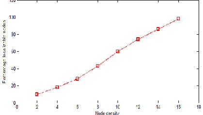
[image:5.595.58.276.74.215.2]Let us first find out the amount of nodes that will be localized according to the distribution of WSN nodes in a deployment area. As already seen in the above fig (2) we create random deployment of nodes using the uniform distribution. With the increase in node density it is obvious that the percentage of localizable nodes will increase steadily. In figure (3) it is shown that upto node density of 8 the percentage of localizable nodes is within fifty percent and after that percentage of localizable nodes increases steeply with increase in node density..
Fig 3: Shows how the percentage of localizable nodes increases for uniform distribution.
5.2.2 Anchor Nodes:
We can see in figure (4) that with the increasing number of anchor nodes the percentage number of localizable nodes increase, that too in both cases of node density of 8 and 10 respectively. The number of anchor nodes to be taken depends on the type of algorithm we are using. If we are using a centralized approach then the then the number of anchors used will be large enough, whereas in case of distributed iterative approach the number of anchor nodes will be less. In a network deployment it is not feasible to keep more number of anchor nodes because of the cost criteria. In DLGR we keep only three anchors for the start of iterative trilateration. From graph of figure (4) it is clear that when the number of anchor nodes in the sensor network deployment is greater than 40 percent then 90 percent and above nodes should be localized.
Fig 4: Depicting anchor nodes v/s percentage of localizable nodes
5.2.3 Sensing Radius
[image:5.595.313.525.310.445.2]According to the unit disk graph model the sensing radius must be within the R i.e. the maximum radius using which the WSN nodes will communicate with each other. Figure (5) shows that as we increase communication radius by ten units from 100 to 200 the percentage of node localizable increases and when max R is reached all nodes are supposed to be localized.
Fig 5: Depicting communication radius v/s percentages of localizable nodes
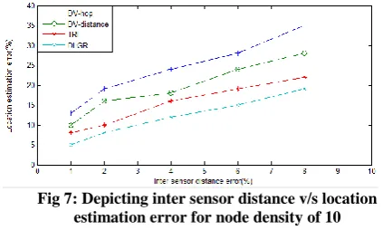
5.3 Location Estimation Error
In our algorithm we are dealing with the noisy inter sensor data. The noise model used is
𝑑𝑒𝑟𝑟 = 𝑑(1 + 𝜌 ∗ 𝑛)
Where 𝑑𝑒𝑟𝑟=noisy distance
d= actual distance 𝜌= 0.1
n= noise levels in percentage
[image:5.595.54.264.377.496.2]Fig 6: Depicting inter sensor distance error v/s location estimation error for node density of 8
Fig 7: Depicting inter sensor distance v/s location estimation error for node density of 10
6. CONCLUSION AND FUTURE WORK
The WSN localization is an NP- hard problem. We have used the concept of rigid graphs to localize the sensor network nodes. In our approach, we used the distributed approach of sensor network localization, where a whole sensor network deployment graph is sub-divided into patches of triangles and quadrilaterals. From the concepts of rigidity theory it is clear that triangles and quadrilaterals falls into the category of Generically Globally Rigid (GGR) graphs. We have made the sensor network graph deployment in the R2 plane (2-dimensional plane) where the Euclidean distances between the different nodes which are connected are known. We have a method which localizes WSN nodes efficiently when there is error in the measurement of the inter sensor distances. We have seen that the measurement errors do not propagate into the output of sensor coordinates. The new algorithm is robust against measurement noise. In this work we used the trilateration graphs by decomposing the sensornet graph into sub-graphs. On these sub-graphs trilateration method is applied to find the WSN sensor node positions. Homogeneous coordinate transformations are applied to position nodes from local coordinate system to global coordinate system.
Possible future perspective from this methodology of sensor network localization includes:
Complete analysis of flip ambiguity which occurs in a GGR graphs when reflection of the coordinates is done of the graph.
Designing a hybrid version of our method which involves centralised as well as distributed version, which might be a need in the future, based on the applications. Sensor network localization using graph rigidity is a new
area in research. Hence the concepts are used and only simulated results have been obtained so far. Therefore, in near future implementing on physical sensor networks have to be done.
7. REFERENCES
[1] L.Moore, J.Leonard, D.Rus, and S.Teller, “Robust Distributed Network Localization with Noisy Range Measurements”, In Proceedings of the Conference on Embedded Networked Sensor Systems (SenSys), ACM, 50–61, 2004.
[2] Y.Shang, and W.Ruml, “Improved MDS-based localization”, In Proceedings of the IEEE Infocom Conference. IEEE Computer Society, 2640–2651, 2004. [3] Y.Koren, C.Gotsman and M.Ben-Chen, “Patchwork:
Efficient localization for sensor networks by distributed global optimization”, Tech. rep, 2005.
[4] J. Aspnes, T. Eren, D. K. Goldenberg, A. S. Morse, W. Whiteley, Y. R. Yang, B. D. O. Anderson and P. N. Belhumeur, “A Theory of Network Localization”, IEEE Trans. Mobile Comput., vol. 5, no 12, pp. 1663–1678, 2006.
[5] J. Aspnes, D. Goldenberg, and Y. R. Yang, “On the Computational Complexity of Sensor Network Localization”, in Proc. ALGOSENSORS 2004, LNCS 3121, pp. 32–44, 2004.
[6] T. Eren, D. K. Goldenberg, W. Whiteley, Y. R. Yang, A. S. Morse, B. D. O. Anderson, and P. N.Belhumeur, “Rigidity, Computation, and Randomization in Network Localization”, in IEEE INFOCOM 2004, vol. 4, 2004, pp. 2673–2684.
[7] A. Savvides, C.C. Han, and M. B.Srivatsava, ”Dynamic fine-grained localization in ad-hoc networks of sensors”. Proc. MobiCom 2001.
[8] R.Connelly, “Generic global rigidity”, Discr. Comput. Geom. 33, 4, 549–563, 2005.
[9] S.Gortler, A.Healy and D.Thurston, “Characterizing generic global rigidity”, arXiv:0710.0926, 2008.
[10] B.D.O.Anderson, A.Shames, G.Mao, “Fomal Theory of Noisy Sensor Network Localization”, Society for Industrial and Applied Mathematics, 2009.
[11] J.Fang, A. S. Morse, “Merging Globally Rigid Graphs and Sensor Network Localization”, Joint 48th IEEE Conference on Decision and Control and 28th Chinese Control Conference Shanghai, P.R. China, December 16-18, 2009.
[12] R.Connelly, “Generic global rigidity”, Available at
http://www.math.cornell.edu/˜conelly, Oct. 2003.
[13] Z. Yang, Y. Liu, and X.Y. Li, “Beyond Trilateration: On the Localizability of Wireless Ad–Hoc Networks,” in IEEE INFOCOM 2009, 2009, pp. 2392–2400.
[14] Z. Zhu, A. M.-C. So, and Y. Ye, “Universal Rigidity and Edge Sparsification for Sensor Network Localization”, 2009.
[15] D. Goldenberg, A. Krishnamurthy, W. Maness, Y. R. Yang, A. Young, A. S. Morse, A.Savvides, and B. Anderson, “Network localization in partially localizable networks,” in Proc. IEEE INFOCOM, 2005, vol.1, pp. 313–326.
[image:6.595.54.266.232.359.2][17] G. Laman, “On graphs and rigidity of plane skeletal structures,” J. Eng. Math., vol. 4, pp.331–340, 1970.
[18] G. Mao, B. Fidan, and B. D. O. Anderson, “Wireless sensor network localization techniques,” Computer Networks, vol. 51, pp. 2529–2553, 2007.
[19] D.K. Goldenberg, P. Bihler, M .Cao, J. Fang, B.D.O. Anderson, A.S. Morse and Y.R. Yang, “Localization in Sparse Networks using Sweeps", Proceedings of the
Seventh International Conference on Mobile Ad Hoc Networking and Computing (Mobicom), 2006.
[20] A. Singer, “A remark on global positioning from local distances”, Proc.Nat. Acad. Sci. 105, 28, 9507–9511, 2008.
[21] W.Fang, G.Yang, “Improvement Based on DV-Hop Localization Algorithm of Wireless Sensor Network”, International Conference on Mechatronic Science, 2011.