Duopolistic Competition and Capacity Choice with Jump Diffusion Process

http://dx.doi.org/10.4236/jmf.2015.52018

Duopolistic Competition and Capacity

Choice with Jump-Diffusion Process

Danmei Chen1,2

1_{School of Finance, Shanghai University of Finance and Economics, Shanghai, China} 2_{Basic Department, Shanghai Jianqiao University, Shanghai, China}

Email: [email protected]

Received 12 April 2015; accepted 17 May 2015; published 22 May 2015

Copyright © 2015 by author and Scientific Research Publishing Inc.

This work is licensed under the Creative Commons Attribution International License (CC BY). http://creativecommons.org/licenses/by/4.0/

Abstract

This paper studies the effects of sudden events on the optimal timing and capacity choice in a du-opoly market. According to the characteristics of economic environment, we assume that the product demand follows geometric Brownian motion with a Poisson jump process. Under the set-tings, the firms face the risk of a sudden drop in demand which is caused by sudden events. We develop the real option game model to derive the investment equilibrium strategies. Moreover, the effects of sudden events on investment decisions are obtained by numerical analysis.

Keywords

Investment Decisions, Competitive, Real Option Game, Jump-Diffusion Process

1. Introduction

We develop the real option game model to discuss the effects of sudden events on the optimal timing and capac-ity choice in a duopoly market. When sudden events occur, such as the financial crisis, economic policy from government, and the emergence of new products, discontinuous change in product demand appears. We use jump- diffusion process to capture the discontinuous changes of product demand.

Most real option game models suppose that the uncertainty variables such as asset price or product demand follow the geometric Brown motion (GBM) to describe the characteristics of continuous changes (e.g. Smets [1]; Dixit and Pindyck [2]; Grenadier [3]; Weeds [4]; Mason and Weeds [5]).

stock price follows a jump-diffusion process with Poisson jump to model sudden events. Kou [9] proposed a double exponential jump-diffusion model. Mason and Wilmot [10] investigated the potential presence of jumps in natural gas price. Ko et al. [11] established real option game model with jump process to investigate the ef-fects of sudden events on investment timing. Pereira and Armada [12] assumed that the entrance of the hidden rivals follows a Poisson process. The project value of the positioned firm has a sudden drop as the hidden rivals enter the market. They presented a model suitable for investment decisions under a hidden competition envi-ronment. Pereira and Rodrigues [13] assumed that firms face the risk of demonopolization from government that can occur as a random or a certain event. They studied the optimal timing in finite-lived monopolies.

The large majority of real option game models focus on the investment timing without considering production capacity choice. However, in reality, production capacity decision is a key factor when one firm invests products. Few studies have considered the interaction between the investment timing and the production capacity in a real option framework. Besanko et al. [14] considered the investment decisions of the heterogeneous products under discrete time framework. Jou and Lee [15] assumed that all firms use the same investment strategy, obtaining the investment timing and the optimal capacity under imperfect competition. Huisman and Kort [16] provided a dynamic analysis of entry deterrence strategies, they discovered the leader overinvest in capacity in order to de-lay entry of the follower. The paper has close connection with these studies, which are extended by introduc-ing the effects of sudden events and pre-emptive competition on the investment decisions. In this model, two firms are allowed to produce the homogeneous products; the product demand is assumed to obey the geometric Brown motion with a Poisson jump process. We discuss strategic investment decisions under duopolistic com-petition.

The remainder of the paper is organized as follows. Section 2 introduces the basic assumption of the real op-tion game model. In Secop-tion 3, we derive the equilibrium strategies in a duopoly market. Secop-tion 4 exercises numerical analysis. Section 5 concludes the paper.

2. Basic Assumption of Real Option Game Model

In the section, we assume two firms have the chance to produce the homogeneous products in a duopoly market. Time is continuous and horizon is infinite. So every firm can defer the investment timing until the optimal mo-ment to enter the market. The firm that enters first is known as the leader and the other as the follower. The product price at timetin market is given as follows:

(

)

t t

P = X a Q− (1) where Xt is the exogenous demand shock, Q is the total market output, unit production cost is c, so the total

costs of production are cQ. Similar to Huisman and Kort [16], every firm cannot adjust production capacity after entering the market and the two firms must make full use of production capacity. The exogenous demand shock is affected by sudden events of external market environment. Suppose that Xt obey thegeometric Brown mo-tion with the Poisson jump process:

dXt=µX ttd +σX Ztd t+θX qtd t

Among the above factors, µ represents the drift rate, σ represents the volatility, dZt is the increment of a standard Brownian motion. We assume ρ µ> to ensure that the option is exercised within a finite period of time. We assume random sudden events follow the Poisson jump process of intensity λ. This means sudden events occur with probability λdt during the time interval dt. Sudden drop in product demand as the events occur. θ represents the deterministic amplitude of the downward jumps satisfying 1− ≤ ≤θ 0. Assume dqt and dZt are independent, so E

(

d dq Zt t

)

=0:

1, with probability d d

0, with probability 1 d t

t q

t

λ λ 

=  ₋



3. Investment Decisions in a Duopoly Market

3.1. The Follower’s Value Function

We need to consider the game backwards. When the leader has invested the project, the follower can make his decisions optimally in response to capacity of the leader. Suppose that the leader has invested the project with capacity ql, the investment threshold and capacity of the follower are chosen as Xf and qf, so the investment costs are cqf. The value function of the follower Vf

(

X q, f

)

is recorded as Vf

( )

X for short. By using the stan-dard real option method, the Bellman equation can be expressed as:

( )

d

(

d

( )

)

.

f f

V X t E V X

ρ =

According to Itô’s Lemma, the value of the follower Vf

( )

X satisfies the following differential equation:

( )

( )

2 2 2

( )

(

(

)

)

( )

2 1

1 .

2

f f

f f f

V X V X

V X X X V X V X

X X

ρ =µ ∂ + σ ∂ +λ +θ −λ

∂ ∂ (2)

The general solution of (1) is of the form:

( )

1 2

1 2 .

f

V X =A Xβ +A Xβ (3) Among them, A1, A2 are the undetermined coefficients, β1, β2 are the roots of the equation

(

)

1

2 2 2

1 1

1 0

2 2

β

σ β +_µ− σ β λ_ + +θ − − =λ ρ

  :

(

)

(

1

)

2

2 2 2

1 2

1 1

2 1

2 2

1, β

µ σ µ σ σ λ ρ λ θ

β

σ

   

−_ − _+ _ − _ + + − +

   

= >

(

)

(

2

)

2

2 2 2

2 2

1 1

2 1

2 2

0. β

µ σ µ σ σ λ ρ λ θ

β

σ

   

−_ − _− _ − _ + + − +

   

= <

Moreover, the value of the follower Vf

( )

X must satisfy three boundary conditions:

( )

0 0, f

V = (4)

( ) (

l f

)

f f ,

f f f

a q q q X

V X cq

ρ µ λθ

− −

= −

− − (5)

( )

(

)

. f

l f f

f

X X

a q q q

V X

X ₌ ρ µ λθ

− − ∂

=

∂ − − (6)

Condition (4) says that the value will be 0 if X =0. Condition (5) and (6) are the value-matching and the smooth-pasting conditions. The two conditions ensure that Vf

( )

X can be maximized when the firm invests at the threshold Xf.

Under these conditions, the value Vf

( )

X , the investment threshold Xf and capacity qf of the follower are calculated as follows:

( )

₍

₎

1 1

, f

f _{l f f}

f f

A X X X

V X _{a q q q X}

cq X X

β

ρ µ λθ

 < 

=  − −

− ≥



− − 

(7)

where

(

)

(

)

1 1

, 1

f

l f

c X

a q q

ρ µ λθ β

β

− − =

(

)

1

1 1

1

.

l f f

f a q q q

X A

β

β ρ µ λθ

− _{− −}

=

− − (9)

We assume that the initial demand level is sufficientlylow, the follower will not start production immediately. According to (7), the value of the follower Vf

( )

X :

( )

1

1 f

V X = A Xβ (10) See from (10), Vf

( )

X is function of qf. We apply (8), (9) to (10), the follower considers the capacity to maximize the value, Vf

( )

X satisfies the first order condition:

( )

*

0. f f f

f _{q q}

V X

q ₌

∂

=

∂ (11)

Combining (8) and (11), we obtain the optimal threshold and the capacity of the follower:

(

)

* * 1

1 1

1 ,

1 1

l

f f

l c a q

q X

a q

ρ µ λθ β

β β

− −

− +

= =

+ − − (12)

Substitute (12) into (9) and (10), the value of the follower

(

_, *

)

f f

V X q is as follows:

(

)

₍

(

₎₍

)

1

₎

1

₍

₎

1

* 1

1 1 1

1 ,

1 1 1

l l

f f

c a q X a q

V X q

c

β

β β

β

β β β ρ µ λθ

 

−  −  −

= _{   }

− + _ + _{ } − − _ (13)

Let ql =0 in (12), the optimal threshold Xm ∗

and the capacity qm ∗

of the monopolist are as follows:

(

)

1

1 1

1 ,

1 1

m m

c a

q X

a

ρ µ λθ β

β β

∗ ₌ ∗₌ + − −

+ − (14)

3.2. The Leader’s Value Function

When the follower is out of the market, the leader earns profits

(

a q q X− l

)

l t at time t. When the follower en- ters the market, the leader’s profits decreases to

(

a− −ql q*f

)

q Xl t at time t. Suppose that the value function of

the leader is V X q_l

(

, _l

)

. V X q_l

(

, _l

)

is also written as V Xl

( )

for simplicity. Let V Xl

( )

=v Xl

( )

−cql, so

( )

l

v X represent that the value subtract the investment costs when the leader has invested. v Xl

( )

satisfies the following differential equation:

( )

( )

2 2 2

( )

(

(

)

)

( ) (

)

2 1

1 .

2

l l

l l l l l

v X v X

v X X X v X v X a q q X

X X

ρ =µ ∂ + σ ∂ +λ +θ −λ + −

∂ ∂ (15)

The general solution of (15) is of the form:

( )

1 2

(

)

1 2

l l l

a q q X v X B Xβ B Xβ

ρ µ λθ −

= + +

− − (16)

The value of the leader V Xl

( )

must satisfy two boundary conditions:

( )

0 0, l

v = (17)

( ) (

*

)

.

l f l f

l f

a q q q X v X

ρ µ λθ

∗ ∗

− − =

− − (18)

If we apply (17), (18) to (16), v Xl

( )

is given by:

( )

1

(

)

1 ,

l l l

a q q X v X B Xβ

ρ µ λθ −

= +

− − (19)

1 1 1 . l f f q q

B X β

ρ µ λθ

∗

∗ −

= −

− − (20)

Before the leader invests the project, the value of the leader V Xl

( )

satisfies the following differential equa-tion:

( )

( )

2 2 2

( )

(

(

)

)

( )

2 1

1 .

2

l l

l l l

V X V X

V X X X V X V X

X X

ρ =µ ∂ + σ ∂ +λ +θ −λ

∂ ∂ (21)

The general solution of (21) is of the form:

( )

1 2

1 2

l

V X =C Xβ +C Xβ (22) In addition, the value of the leader V Xl

( )

must satisfy three boundary conditions:

( )

0 0, l

V = (23)

( ) (

l

)

l l l 1 l f f ,

l l l

f

q q X

a q q X X

V X cq

X β

ρ µ λθ ρ µ λθ

∗ ∗

∗

 

−

= −_ _ −

− − _{ } − − (24)

( )

(

)

11

1

. l

l f f l l

l l

f f

X X

q q X a q q

V X X

X X X

β

β

ρ µ λθ ρ µ λθ

− _{∗ ∗} ∗ ∗ =   − ∂ = − _ _

∂ − − _{ } − − (25)

Condition (24) says that:

( )

( )

.

l l l l l

V X =v X −cq (26) If we apply (23), (24), (25) to (22), we obtain:

( ) (

)

(

)

1 1 1 * , l

l f f l l

l l l f

f

l f l

l f

C X X X

q q X a q q X X

V X cq X X X

X

a q q q X

cq X X

β

β

ρ µ λθ ρ µ λθ

ρ µ λθ

∗ ∗

∗

∗

∗



 _< 

 _{ }

− 

= _{− −} −_ _{ − −} − ≤ <

    − −  _{− ≥}  _{− −}  (27) where

(

)

1 1 , 1 l l c X a q

ρ µ λθ β

β

− − =

− − (28)

(

)

1

1

1 _{* *}

1

1

1 * *

1

.

l f f l l

l l

f f

q q X a q q

X X

C

X X

β

β _β

β ρ µ λθ ρ µ λθ

− −  _{−  }    = − _ _  − − _{ } − −    (29)

We assume that the initial demand level is sufficiently low, the leader will not start production immediately. To maximize the value, we apply (28), (29) to (27), and substitute (12) into (27), the value of the leader is cal-culated as:

( )

₍

₎

1

1 1 1

1 1

1 1 1

1 1

1 1

l l

l

cq X a q

V X

c

β

β β β

β β

β β β ρ µ λθ

 _{  }

 −  _   _ −

= ₋   − ₊   _{− −} 

   

  _   _  (30)

3.3. Equilibrium

means that one firm is designated as the leader beforehand. So, the risk of pre-emption is eliminated, two firms can delay their investment to maximize their values. When the initial demand is sufficiently low, we suppose the leader (follower) select the optimal capacity qln

∗

( )

fn

q∗ , the investment threshold Xln

∗

( )

fn

X∗ . Thus, the value of the leader (follower) is denoted as V X q_l

(

, _ln∗

)

(

Vf

(

X q, fn

)

)

∗

.Similar to the above, V Xl

( )

must satisfy:

( )

0.

l ln

l

l q q

V X

q ₌∗ ∂

=

∂ (31)

Combining (28) and (31), we have:

(

)

1 1 1 1 , . 1 1

ln m ln m

c a

q q X X

a

ρ µ λθ β

β β

∗ ₌ ∗ ₌ ∗ ₌ ∗ ₌ + − −

+ − (32)

So, by substituting (32) into (12), the optimal threshold and the capacity of the follower are given by:

(

)

(

) (

(

)

)

(

)

2 1

1 1

2

1 1 1 1 1

1 1

,

1 1 1 1

ln

fn fn

ln

c c

a q a

q X

a a q

ρ µ λθ β ρ µ λθ

β β

β _β β β β

∗ ∗ ∗ ∗ − − + − − − + = = = =

+ + − − − (33)

Comparing (14) and (32), Proposition 1 is obtained.

Proposition 1. The investment threshold of the designated leader is the same as that of the monopolist.

The designated leader has valuable option to defer investment at the optimal threshold of the monopolist as he need not face the risk of being preempted.

However, two firms are allowed to invest first in reality. This means that firm roles are endogenous. So, the risk of pre-emption exists. We assume that the initial demand level is sufficiently low, two firms are induced to delay their investment. When firm roles are endogenous, according to Fudenberg and Tirole [17], if one firm in-tends to invest at the threshold Xm

∗

first, the other firm will pre-empt it as long as the value of the firm is greater than that of the other firm. So the value is equal for both firms in equilibrium. Suppose that the value of the leader (follower) V X q_l

(

, _le∗

)

(

Vf

(

X q, fe

)

)

∗

, the optimal capacity qle

∗

( )

fe

q∗ , the investment threshold Xle ∗

( )

Xfe ∗

. So,

(

,

)

(

,

)

.

l le f fe

V X q∗ =V X q∗ (34)

Proposition 2 describes the sequential equilibrium. For the proof of Proposition 2, see the Appendix. Proposition 2. (sequential equilibrium). If the initial demand level is lower than Xle

∗

, the equilibrium in-vestment is sequential, the leader invests with capacity qle

∗

until the demand Xt reaches Xle ∗

, the follower invests with capacity qfe

∗

until the demand Xt reaches Xfe ∗

. Where, the optimal capacity of the leader qle ∗

is a unique solution of the equation:

1 1 1

1 1

1 1 1

1 0,

1 le 1 1

a q

β β

β β

β β β

+ ∗  _{ }  _{ }  −_{ }  −_{ } = + + +         (35)

the optimal capacity Xle ∗ :

(

)

1 1 , 1 le le c X a q

ρ µ λθ β β ∗ ∗ − − =

− − (36)

the optimal capacity qfe ∗

and investment threshold qfe ∗

of the follower:

(

)

1 1 1 1 , . 1 1 le fe fe le c a q q X a q

ρ µ λθ β β β ∗ ∗ ∗ ∗ − − − + = =

+ − − (37)

Proposition 3, 4 describe the impacts of pre-emptive competition. The proofs are in Appendix.

Proposition 3. When the risk of pre-emption exists, the leader reduce its capacity to invest early, the follower increases its capacity to invest early. That is, qle qln

∗ _< ∗

, Xle Xln ∗_< ∗

, qfe qfn ∗ _> ∗

, Xfe Xfn ∗ _< ∗

. Proposition 4.If the initial demand level is lower than Xle

∗

(

,

) (

,

)

l le l ln

V X q∗ <V X q∗ , V_f

(

X q, ∗_fe

)

>V_f

(

X q, ∗_fn

)

.

4. Numerical Results Analysis

4.1. The Impacts of Pre-Emptive Competition

The subsection describes the impacts of pre-emptive competition on the firms. The parameters are as follows: 0.05

ρ= , µ=0.03, c=10, a=1, λ =0.1, θ = −0.1, σ =0.3.

Based on the given parameters, we calculate to obtain the optimal capacities and thresholds respectively as the roles of the firms are endogenous or exogenous: Xln 1.9427

∗ ₌

, Xfn 3.3656 ∗ ₌

, qln 0.4228 ∗ ₌

, qfn 0.2440 ∗ ₌

, 1.5456

le

X∗ = , Xfe 2.6776 ∗ ₌

, qle 0.2745 ∗ ₌

, qfe 0.3067 ∗ ₌

. We can see that Xle Xln ∗ _< ∗

, qle qln ∗ _< ∗

hold from the numerical results. This means that the leader will reduce production to speed up the investment due to fear of being pre-empted. Comparison of the numerical results, we find that Xfe Xfn

∗ _< ∗

, qfe qfn ∗ _> ∗

[image:7.595.200.427.502.707.2]

stand. This is be-cause when the leader reduces production to invest ahead, the production in the market is not enough, the price is relatively high, the follower is willing to increase production to invest ahead. These results indicate pre-emptive competition makes the two firms to accelerate investment.

Figure 1 further shows the relationship between the values of the two firms as the roles are endogenous or

exogenous. The numerical analysis is based on the assumptions that the initial demand is less than Xle ∗

, the firms will wait until the optimal timing to enter the market. See Figure 1, the value of the designated leader is the largest, that of the leader is the second, that of the designated follower is the smallest. That is to say,

(

,

)

(

,

) (

,

)

f fn f fe l ln

V X q∗ <V X q∗ <V X q∗ . When the firm roles are designated, the designated follower is at a disad-vantage in the game. The designated leader is dominant, he will invest at the optimal timing not considering the risk of pre-emption. So, the conclusion is intuitive.

So, Figure 1 suggests the conclusions of Proposition 3, 4.

4.2. Sensitivity Analysis

In the subsection, we perform a comparative static analysis, focusing on the impacts of different parameter val-ues such as the Poisson jump process of intensity λ, the deterministic amplitude of the jumps θ, the volatility σ .

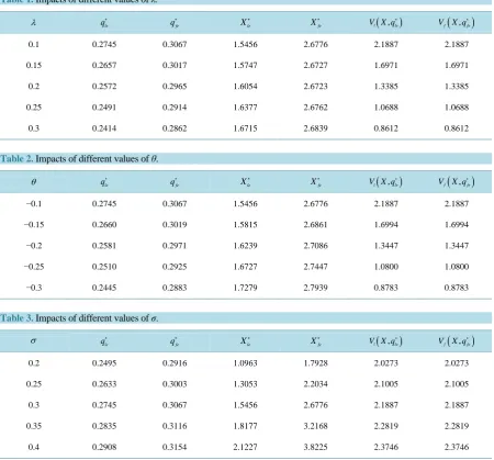
Table 1illustrates the impacts of different values of λ. The parameters are as follows: ρ=0.05, µ=0.03,

10

c= , a=1, X =1, θ = −0.1, σ =0.3. The intensity λ measures the arrival probability of sudden events such as financial crisis or financial tsunami.When sudden events occur, the economy will be immersed in de-pression, a sudden decline in market demand. When λ increases,the leader will reduce its production to invest later, the follower will reduce its production to invest earlier first, then later. Increasing λ brings more risks which will make the leader more conservative. The investment threshold of the follower is non monotonic with

λ. As we mentioned above, higher λ makes the investors reduce output to invest later. On the other hand, higher price which due to less output encourages the follower to invest earlier. As λ increases, the values of both the leader and the follower will decline.

Table 2illustrates the impacts of different values of θ. The parameters are as follows: ρ=0.05, µ=0.03,

10

[image:8.595.89.540.301.720.2]

c= , a=1, X =1, λ =0.1, σ =0.3. The deterministic amplitude of the jumps θ measures the level of the effect of the sudden events on investment environment. As θ decreases, both the leader and the follower will re-duce production to invest later. Decreasing θ means worse investment environment. Thus, the values of both will decline.

Table 3illustrates the impacts of different values of σ. The parameters are as follows: ρ=0.05, µ=0.03,

10

c= , a=1, X =1, λ =0.1, θ = −0.1. As σ increases, the uncertainties and risks linked with investment also increase. When the uncertainties and risks rise, both the leader and the follower will prefer to wait for better chance rather than now. So, they will increase production to invest later, the values of both will increase.

5. Conclusions

In this paper, we examine the impact of sudden events on the investment timing and production capacity deci-sions of a firm that faces competition. We obtain the investment equilibrium strategies.

Table 1. Impacts of different values of λ.

λ qle

∗

fe

q∗ Xle

∗

fe

X∗ V X ql

(

, le

)

∗

(

)

,

f fe

V X q∗

0.1 0.2745 0.3067 1.5456 2.6776 2.1887 2.1887

0.15 0.2657 0.3017 1.5747 2.6727 1.6971 1.6971

0.2 0.2572 0.2965 1.6054 2.6723 1.3385 1.3385

0.25 0.2491 0.2914 1.6377 2.6762 1.0688 1.0688

0.3 0.2414 0.2862 1.6715 2.6839 0.8612 0.8612

Table 2. Impacts of different values of θ.

θ qle

∗

fe

q∗ Xle

∗

fe

X∗ V X ql

(

, le

)

∗

(

)

,

f fe

V X q∗

−0.1 0.2745 0.3067 1.5456 2.6776 2.1887 2.1887

−0.15 0.2660 0.3019 1.5815 2.6861 1.6994 1.6994

−0.2 0.2581 0.2971 1.6239 2.7086 1.3447 1.3447

−0.25 0.2510 0.2925 1.6727 2.7447 1.0800 1.0800

−0.3 0.2445 0.2883 1.7279 2.7939 0.8783 0.8783

Table 3. Impacts of different values of σ.

σ q_le∗ qfe

∗

le

X∗ Xfe

∗

(

)

,

l le

V X q∗ Vf

(

X q, fe

)

∗

0.2 0.2495 0.2916 1.0963 1.7928 2.0273 2.0273

0.25 0.2633 0.3003 1.3053 2.2034 2.1005 2.1005

0.3 0.2745 0.3067 1.5456 2.6776 2.1887 2.1887

0.35 0.2835 0.3116 1.8177 3.2168 2.2819 2.2819

We find that pre-emptive competition and sudden events have great influence on investment decisions; pre-emptive competition makes firms accelerate investment. Higher uncertainty for market demand increases the values of both the leader and the follower. When sudden events occur more frequently or product demand de-clines in greater magnitude, the values of both firms will decline.

This paper considers the case of two firms. Consequently, a natural idea is to consider the case of a number of firms. Future researchcan also be concerned withtheapplication of a different randomprocess, e.g., arithmetic Brownian motion.

Acknowledgements

This research is supported by NSFC (71271127, 10971127).

References

[1] Smets, F. (1991) Exporting versus FDI: The Effect of Uncertainty, Irreversibilities and Strategic Interactions. Working

Paper, Yale University, New Haven.

[2] Dixit, A. K. and Pindyck, R.S. (1994) Investment under Uncertainty. Princeton University Press, Princeton.

[3] Grenadier, S.R. (1996) The Strategic Exercise of Options: Development Cascades and Overbuilding in Real Estate

Markets. The Journal of Finance, 51, 1653-1679. http://dx.doi.org/10.1111/j.1540-6261.1996.tb05221.x

[4] Weeds, H. (2002) Strategic Delay in a Real Options Model of R&D Competition. The Review of Economic Studies, 69,

729-747. http://dx.doi.org/10.1111/1467-937X.t01-1-00029

[5] Mason, R. and Weeds, H. (2010) Investment, Uncertainty and Pre-Emption. International Journal of Industrial

Or-ganization, 28, 278-287. http://dx.doi.org/10.1016/j.ijindorg.2009.09.004

[6] Jorion, P. (1988) On Jump Processes in the Foreign Exchange and Stock Markets. Review of Financial Studies, 1, 427-

445. http://dx.doi.org/10.1093/rfs/1.4.427

[7] Bates, D.S. (1996) Jumps and Stochastic Volatility: Exchange Rate Processes Implicit in Deutsche Mark Options.

Re-view of Financial Studies, 9, 69-107. http://dx.doi.org/10.1093/rfs/9.1.69

[8] Merton, R.C. (1976) Option Pricing When Underlying Stock Returns Are Discontinuous. Journal of Financial

Eco-nomics, 3, 125-144. http://dx.doi.org/10.1016/0304-405X(76)90022-2

[9] Kou, S.G. (2002) A Jump-Diffusion Model for Option Pricing. Management Science, 48, 1086-1101.

http://dx.doi.org/10.1287/mnsc.48.8.1086.166

[10] Mason, C.F. and Wilmot, N.A. (2014) Jump Processes in Natural Gas Markets. Energy Economics, 46, S69-S79.

http://dx.doi.org/10.1016/j.eneco.2014.09.015

[11] Ko, C.-C., Lin, T.T. and Yang, C. (2011) The Venture Capital Entry Model on Game Options with Jump-Diffusion

Process. International Journal of Production Economics, 134, 87-94. http://dx.doi.org/10.1016/j.ijpe.2011.02.016

[12] Pereira, P.J. and Armada, M.R. (2013) Investment Decisions under Hidden Competition. Economics Letters, 121, 228-

231. http://dx.doi.org/10.1016/j.econlet.2013.07.029

[13] Pereira, P.J. and Rodrigues, A. (2014) Investment Decisions in Finite-Lived Monopolies. Journal of Economic Dyna

-mics and Control, 46, 219-236. http://dx.doi.org/10.1016/j.jedc.2014.07.003

[14] Besanko, D., Doraszelski, U., Lu, L.X. and Satterthwaite, M. (2010) Lumpy Capacity Investment and Disinvestment

Dynamics. Operations Research, 58, 1178-1193. http://dx.doi.org/10.1287/opre.1100.0823

[15] Jou, J.B. and Lee, T. (2008) Irreversible Investment, Financing, and Bankruptcy Decisions in an Oligopoly. Journal of

Financial and Quantitative Analysis, 43, 769-786. http://dx.doi.org/10.1017/S0022109000004282

[16] Huisman, K. and Kort, P.M. (2013) Strategic Capacity Investment under Uncertainty. Tilburg University, Tilburg.

[17] Fudenberg, D. and Tirole, J. (1985) Preemption and Rent Equalization in the Adoption of New Technology. The

Appendix

The proof for Proposition 2:

When pre-emptive competition exists, the follower makes his decisions reacting to the capacity of the leader. According to (28), we can obtain (36). According to (12), we can obtain (37).

The value is the same for both firms at the threshold ql qle ∗

= . Substitute ql qle ∗

= into (13) and (30), we have:

(

)

(

(

)(

)

)

(

)

1 1 1

1 1 1 1 *

1 1 1

1 1 1 1 1 1

1 1

1

1 1 1 1 1

le

le le c a q X le

cq X a q a q

c c

β β β

β β β β

β β β

β β β ρ µ λθ β β β ρ µ λθ

∗

∗ _{ − }  _{ } _{ −} ∗ _{ −  −   − }

 −   =  

     

−   _  +  _ − −  − +  +   − − 

Simplifying the above equation, we conclude that (35) stands and qle ∗

is a unique root of (35).

The proof for Proposition 3:

We proof that when β >1 1,

1 1 1 1 1 2 β β β   <  ₊ 

  first.

1 1 1 1 1 1 1 1 1 1 1

lim , lim ,

1 2 1 e

β β β β β β β β → →∞     = =  ₊   ₊ 

    (38)

(

)

1

1

1

1 1 1

1

1 1 1 1

1 1

1 1 ln .

1 1 1

β

β

β

β β _β β

β β β β

 

∂  ₊  _{    }

 _{ =  + + }

  _  _

∂ + _ + _{  } + _

Let

( )

1 1

1 1

1 1

ln

1

f β β

β β

 + 

= _{ }−

+

  , we have 1

( )

1 1

1

lim ln 2 0

2 f

β→ β = − > , _βlim_1→∞f

( )

β1 =0, and if β >1 1, then

( )

(

)

(

)

1 2 1 1 1 1 1 0 1 1 f β β β β

′ = − <

+

+ . So, f

( )

β1 >0 . Thus, we conclude

(

)

1 1

1

1 1 ln 0

1

β β

β

 

+ + _{ }<

+

  and 1 1 1 1 1 0 β β β β   ∂  ₊ 

 _{ <}

∂ . According to (38), we obtain that β >1 1,

1 1 1 1 1 2 β β β   <  ₊    .

Substitute qln ∗

into (35), we have

11 1

1 1

1 1 1 1

1 0

1 1 1 1

a a

β β

β β

β β β β

+

 _{ }  _{ }

 −_{ }  −_{ } >

+ + + +

     

 

. So, qle qln ∗ _< ∗

. Combining

(12) and (28),Proposition 3 holds. The proof for Proposition 4: If ql qln

∗

≤ , taking the first derivatives on (13) and (30) respectively:

( )

(

)

(

)

(

)

1 1

1 1 _{1 1}

1 1 1

1 1 1

1 1 1

1 0,

1 1

l l

l

l

c a q a q X

V X

q c

β

β β _{β β}

β _{β β}

β β β ρ µ λθ

−   −  − +    ∂ _{ }  −      = _{ } −_{   } ≥ ∂ −   _  +   _ − − 

(

)

(

)

(

)

1 1 1 1 1 1 , ₁ 0 1 1

f f _l

l

V X q _{cX a q}

q c

β

β β

β

β β ρ µ λθ

∗

∂ _{= −}  −   −  _<

 

 

∂ − _ + _{ } − − _ . So, if ql qln ∗

≤ , V Xl

( )

is a monotonically increas-

ing function of ql, Vf

(

X q, f

)

∗

is a monotonically decreasing function of ql. Because qle qln ∗ _< ∗

, we have